Scientists pumped half a tonne of explosive material into 50km-deep holes spread nearly 100km across New Zealand’s North Island to measure rock layers beneath the surface Photograph: Diana Plater/AAP
Geologists may have finally explained how tectonic plates shift by blowing up hundreds of kilograms of dynamite in New Zealand.
Half a tonne of explosive slurry was pumped into a dozen, steel-cased holes spread nearly 100km across New Zealand’s north island.
The seismic waves produced by the subsequent explosion reached the base of the tectonic plate and rebounded to the surface, where they were recorded by more than 1,000 seismographs.
Because seismic waves encode information about each of the layers they pass through, an international team of researchers was able to use them to produce detailed images of what lies beneath the earth’s surface.
They revealed the existence of a narrow, lubricating layer of rock about 73km deep, over which the plate “skied” several centimetres a year.
The results are published in the latest issue of the scientific journal Nature.
One of the researchers, professor Tim Stern of Victoria University, Wellington, said earlier studies had relied on recording the seismic waves produced by earthquakes.
“But those earthquake waves are very low-frequency, wobbly looking waves, and they haven’t really given us the details we need,” he said.
Detonating 500kg of dynamite – the equivalent of more 2,600 sticks – provided far sharper echoes.
The 50m-deep explosive holes were dug in a line parallel to the border of the Pacific and Australian plates, Stern said. The two plates meet at a relatively shallow 12- to 15-degree angle, making the area ideal for rebounding seismic waves, which he likened to “bouncing light off a mirror”.
Once triggered, the explosion caused the earth to shake and produced a “big whoomp” that could be heard from 10km away. “But that’s about all,” Stern said.
While the discovery of the slippery 10km layer explains how the plates move, what causes them to do so remains unclear.
One leading theory suggests the plates are pulled or pushed along their edges. Another, posits that the plates are connected to a deeper layer of hot, convecting mantle and getting dragged.
Stern said the research showed “there’s still fundamental discoveries to be made” in the theory of plate tectonics, which has dominated earth science since the 1960s.
A forerunner of the idea was suggested in 1912 by a German meteorologist, Alfred Wegener, who observed that the east coast of South America and the west coast of Africa fit together like a puzzle.
He suggested the world’s continents had once been fused together in a supercontinent he named Pangaea (“all the world”), but had since broken up and drifted to their present locations.
Earlier theories had suggested the world’s continents had been connected by massive land bridges, which have since broken off and sunk.
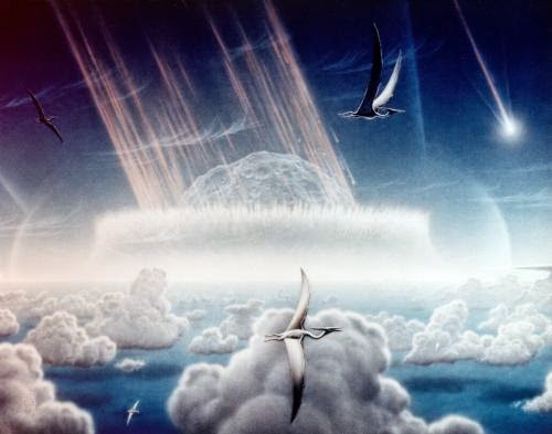
What suddenly made the dinosaurs disappear 65 million or 66 million years ago? Whatever it was, all indications show that it was a massive extinction event. The fossil record not only shows dinosaurs disappearing, but also numerous other species of the era. Whatever it was, there was a sudden change in the environment that changed evolution forever.
The leading theory for this change is a small body (likely an asteroid or a comet) that slammed into Mexico’s Yucatan Peninsula. The impact’s force generated enough debris to block the Sun worldwide, killing any survivors of starvation.
The crater
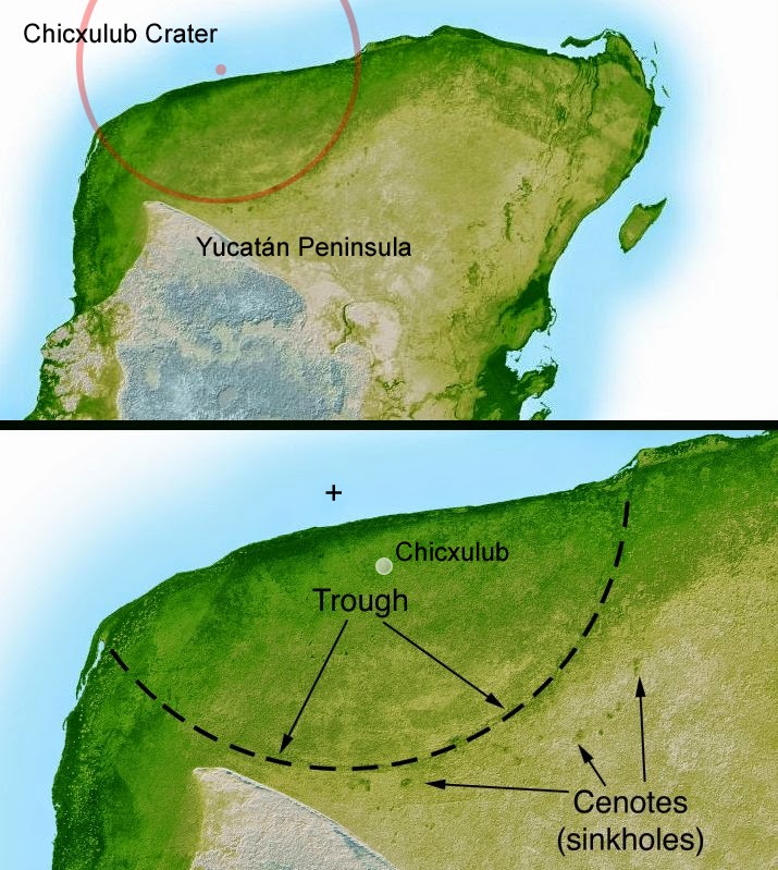
There have been numerous theories proposed for the dinosaurs’ death, but in 1980 more evidence arose for a huge impact on the Earth. This happened when a father-son University of California, Berkeley research team—Luis Alvarez and Walter Alvarez—discovered a link with a 110-mile (177-kilometer) wide impact crater near the Yucatan coast of Mexico. It’s now known as Chicxulub.
Chicxulub crater in Mexico. Credit: Wikipedia/NASA
It sounds surprising that such a huge crater wasn’t found until that late, especially given satellites had been doing Earth observation for the better part of 20 years at that point. But as NASA explains, “Chicxulub … eluded detection for decades because it was hidden (and at the same time preserved) beneath a kilometer of younger rocks and sediments.”
The data came from a Mexican company that was seeking oil in the region. The geologists saw the structure and guessed, from its circular shape, that it was an impact crater. Further observations were done using magnetic and gravity data, NASA said, as well as space observations (including at least one shuttle mission).
The layer
The asteroid’s impact on Earth was quite catastrophic. Estimated at six miles (9.7 kilometers) wide, it carved out a substantial amount of debris that spread quickly around the Earth, aided by winds in the atmosphere.
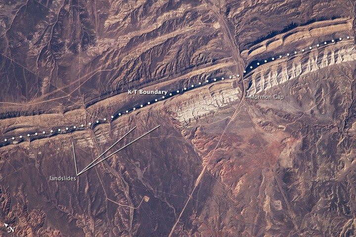
If you look in the fossil record all over the world, you will see a layer that is known as the “K-T Boundary”, referring to the boundary between the Cretaceous and Tertiary periods in geologic history. This layer, says the University of California, Berkeley, is made up of “glassy spheres or tektites, shocked quartz and a layer of iridium-enriched dust.”
K-T Boundary. Credit: NASA Earth Observatory
Of note, iridium is a rare element on the surface of the Earth, but it’s fairly common in meteorites. (Some argue that the iridium could have come from volcanic eruptions churning it up from inside the Earth; for more information, see this Universe Today story.)
Was it simply ‘the last straw’?
While an asteroid (or comet) striking the Earth could certainly cause all the catastrophic events listed above, some scientists believe the dinosaurs were already on their last legs (so to speak) before the impact took place. Berkeley points to “dramatic climate variation” in the million years preceding the event, such as very cold periods in the tropical environment that the dinosaurs were used to.
What might have caused this were several volcanic eruptions in India around the same time. Some scientists believe it was the volcanic eruptions themselves that caused the extinction and that the impact was not principally to blame, since the eruptions could also have produced the iridium layer. But Berkeley’s Paul Renne said the eruptions were more a catalyst for weakening the dinosaurs.
“These precursory phenomena made the global ecosystem much more sensitive to even relatively small triggers, so that what otherwise might have been a fairly minor effect shifted the ecosystem into a new state,” Renne stated in 2013. “The impact was the coup de grace.”
Note : The above story is based on materials provided by Universe Today. The original article was written by Elizabeth Howell.
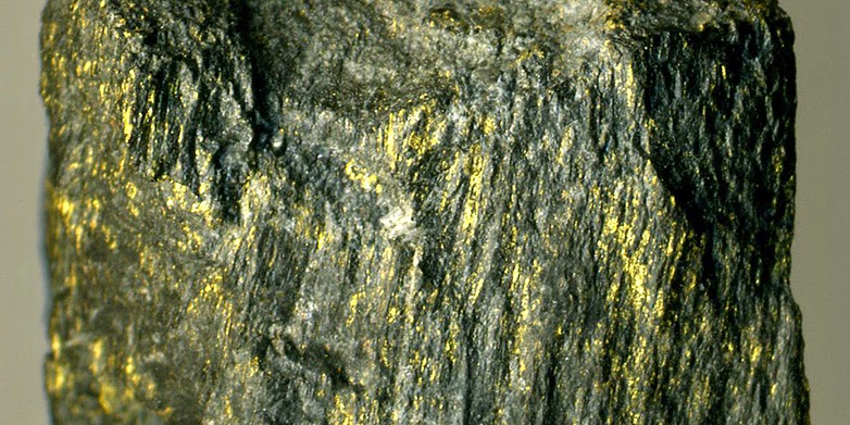
The richest gold ore in Witwatersrand is found in thin layers rich in carbon, plating fibres of ancient microbial life forms. (Photo: James St. John / Wikimedia Commons)
The Witwatersrand Basin in South Africa holds the world’s largest gold deposits across a 200-km long swathe. Individual ore deposits are spread out in thin layers over areas up to 10 by 10 km and contain more gold than any other gold deposit in the world. Some 40% of the precious metal that has been found up to the present day comes from this area, and hundreds of tons of gold deposits still lie beneath the earth. The manner in which these giant deposits formed is still debated among geologists. Christoph Heinrich, Professor of Mineral Resources at ETH and the University of Zurich, recently published a new explanation in the journal Nature Geoscience, trying to reconcile the contradictions of two previously published theories.
The prevailing ‘placer gold’ theory states that the gold at Witwatersrand was transported and concentrated through mechanical means as metallic particles in river sediment. Such a process has led to the gold-rich river gravels that gave rise to the Californian gold rush. Here, nuggets of placer gold have accumulated locally in river gravels in the foothills of the Sierra Nevada, where primary gold-quarz veins provide a nearby source of the nuggets.
But no sufficiently large source exists in the immediate sub-surface of the Witwatersrand Basin. This is one of the main arguments of proponents of the ‘hydrothermal hypothesis’, according to which gold, chemically dissolved in hot fluid, passed into the sediment layers half a billion years after their deposition. For this theory to work, a 10 km thick blanket of later sediments would be required in order to create the required pressure and temperature. However, the hydrothermal theory is contradicted by geological evidence that the gold concentration must have taken place during the formation of host sediments on the Earth’s surface.
Rainwater rich in hydrogen sulphide
Heinrich believes the concentration of gold took place at the Earth’s surface, indeed by flowing river water, but in chemically dissolved form. With such a process, the gold could be easily ‘collected’ from a much larger catchment area of weathered, slightly gold-bearing rocks. The resource geologist examined the possibility of this middle way, by calculating the chemical solubility of the precious metal in surface water under the prevailing atmospheric and climatic conditions.
Experimental data shows that the chemical transport of gold was indeed possible in the early stages of Earth evolution. The prerequisite was that the rainwater had to be at least occasionally very rich in hydrogen sulphide. Hydrogen sulphide binds itself in the weathered soil with widely distributed traces of gold to form aqueous gold sulphide complexes, which significantly increases the solubility of the gold. However, hydrogen sulphide in the atmosphere and sulphurous gold complexes in river water are stable only in the absence of free oxygen. “Quite inhospitable environmental conditions must have dominated, which was possible only three billion years ago during the Archean eon,” says Heinrich. “It required an oxygen-free atmosphere that was temporarily very rich in hydrogen sulphide — the smell of rotten eggs.” In today’s atmosphere, oxygen oxidises all hydrogen sulphide, thus destroying gold’s sulphur complex in a short time, which is why gold is practically insoluble in today’s river water.
Volcanoes and bacteria as important factors
In order to increase the sulphur concentration of rainwater sufficiently in the Archean eon, basaltic volcanism of gigantic proportions was required at the same time. Indeed, in other regions of South Africa there is evidence of giant basaltic eruptions overlapping with the period of the gold concentration.
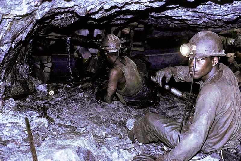
A third factor required for the formation of gold deposits at Witwatersrand is a suitable location for concentrated precipitation of the gold. The richest deposits of gold ore in the basin are found in carbon-rich layers, often just millimetres to centimeters thick, but which stretch for many kilometres. These thin layers contain such high gold concentrations that mining tunnels scarcely a metre high some three kilometres below the Earth’s surface are still worthwhile.
Hard and dangerous labour: The mines provide no place to stand. (Photo: Courtesy Prof. C. Heinrich)
The carbon probably stems from the growth of bacteria on the bottom of shallow lakes and it’s here that the dissolved gold precipitated chemically, according to Heinrich’s interpretation.
The nature of these life forms is not well known. “It’s possible that these primitive organisms actively adsorbed the gold,” Heinrich speculates. “But a simple chemical reduction of sulphur-complexed gold in water to elementary metal on an organic material is sufficient for a chemical ‘gilding’ of the bottom of the shallow lakes.”
The gold deposits in the Witwatersrand, which are unique worldwide, could have thus been formed only during a certain period of the Earth’s history: after the development of the first continental life forms in shallow lakes at least 3 billion years ago, but before the first emergence of free oxygen in the Earth’s atmosphere approximately 2.5 billion years ago.
Reference:
Christoph A. Heinrich. Witwatersrand gold deposits formed by volcanic rain, anoxic rivers and Archaean life. Nature Geoscience, 2015; DOI: 10.1038/ngeo2344
Note : The above story is based on materials provided by ETH Zürich. The original article was written by Peter Rüegg.
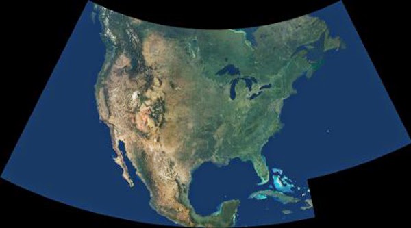
North America traveled in fast company back in its youth.
A new study led by Michigan Technological University geophysicist Aleksey Smirnov reveals that 1.1 billion years ago, the North American tectonic plate scooted along at a blistering 24.6 centimeters—about 10 inches—per year.
While it may not seem to be shattering any speed records, that’s twice as fast as continental plates typically traveled in their wanderings over the earth’s surface back in Precambrian times. Oceanic plates moved that quickly, but they are also much thinner, only 10 to 15 kilometers deep. Continental plates are up to 70 kilometers (43 miles) thick.
These days, tectonic plates—15-20 huge, interlocking pieces that make up the earth’s crust—are even slower. Nevertheless, their movements are partially responsible for geological phenomena like earthquakes, volcanoes and mountain building.
North American Plate
Smirnov’s team made its discovery while investigating a totally different problem. Every time the earth’s magnetic field switches 180 degrees—which happens every few hundred thousand years or so—the change is recorded in certain volcanic minerals that are formed as lava cools. The only apparent exception to the 180-degree rule was found during earlier investigations of the “fossil magnetism” of the rocks in Michigan’s Keweenaw Peninsula. Scientists were surprised to find what looked like a switch of about 200 degrees. In other words, the magnetic north and south poles seemed to be seriously off kilter at one point about a billion years ago.
Smirnov’s group looked at rocks from the same era at the Coldwell Complex, located in Ontario near the town of Marathon. There, a more-complete fossil magnetization record is available. They found that it wasn’t the earth’s magnetic field that had moved so dramatically: it was the North American Plate itself. Their discovery validates an earlier hypothesis that the continent was breaking speed records back in the day.
But what engine could drive a continental plate at such a clip? Smirnov believes the answer may lie deep beneath the surface of the earth.
Mantle Activity
“We know there was a lot of mantle activity at the time,”he said. The mantle is the layer between the earth’s crust and its core. “The continental and oceanic plates float atop this thick layer of semi-molten rock, and at this point in the Precambrian Era all the land masses were drifting together to form the supercontinent Rodinia.
“We had a very vigorous mantle at that time, and that would move this huge continental plate,” said Smirnov.
Reference:
“Paleomagnetism of the ~1.1 Ga Coldwell Complex (Ontario, Canada): Implications for Proterozoic Geomagnetic Field Morphology and Plate Velocities,”coauthored by Smirnov, PhD student Evgeniy Kulakov and Professor Jimmy Diehl, all of Michigan Tech, is published Dec. 21 in the Journal of Geophysical Research: Solid Earth. DOI: 10.1002/2014JB011463
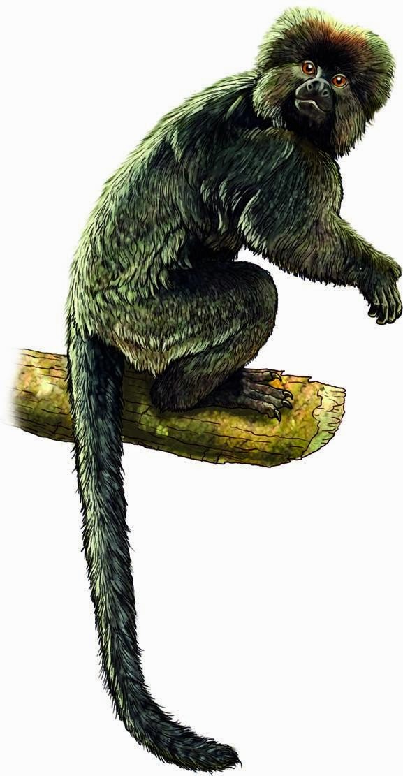
This is an artist rendering of what South America’s oldest known monkey might have looked like. It was about the size of a squirrel, but with a longer tail, and probably weighed less than 250 grams (~0.5 lbs). Credit: Artist: Jorge González
For millions of years, South America was an island continent. Geographically isolated from Africa as a result of plate tectonics more than 65 million years ago, this continent witnessed the evolution of many unfamiliar groups of animals and plants. From time to time, animals more familiar to us today — monkeys and rodents among others — managed to arrive to this island landmass, their remains appearing abruptly in the fossil record. Yet, the earliest phases of the evolutionary history of monkeys in South America have remained cloaked in mystery. Long thought to have managed a long transatlantic journey from Africa, evidence for this hypothesis was difficult to support without fossil data
A new discovery from the heart of the Peruvian Amazon now unveils a key chapter of the evolutionary saga of these animals. In a paper published February 4, 2015 in the scientific journal Nature, the discovery of three new extinct monkeys from eastern Peru hints strongly that South American monkeys have an African ancestry.
Co-author Dr. Ken Campbell, curator at the Natural History Museum of Los Angeles County (NHM), discovered the first of these fossils in 2010, but because it was so strange to South America, it took an additional two years to realize that it was from a primitive monkey.
Mounting evidence came as a result of further efforts to identify tiny fossils associated with the first find. For many years, Campbell has surveyed remote regions of the Amazon Basin of South America in search for clues to its ancient biological past. “Fossils are scarce and limited to only a few exposed banks along rivers during the dry seasons,” said Campbell. “For much of the year high water levels make paleontological exploration impossible.” In recent years, Campbell has focused his efforts on eastern Peru, working with a team of Argentinian paleontologists expert in the fossils of South America. His goal is to decipher the evolutionary origin of one of the most biologically diverse regions in the world.
The oldest fossil records of New World monkeys (monkeys found in South America and Central America) date back 26 million years. The new fossils indicate that monkeys first arrived in South America at least 36 million years ago. The discovery thus pushes back the colonization of South America by monkeys by approximately 10 million years, and the characteristics of the teeth of these early monkeys provide the first evidence that monkeys actually managed to cross the Atlantic Ocean from Africa.
Reference:
Mariano Bond, Marcelo F. Tejedor, Kenneth E. Campbell, Laura Chornogubsky, Nelson Novo, Francisco Goin. Eocene primates of South America and the African origins of New World monkeys. Nature, 2015; DOI: 10.1038/nature14120
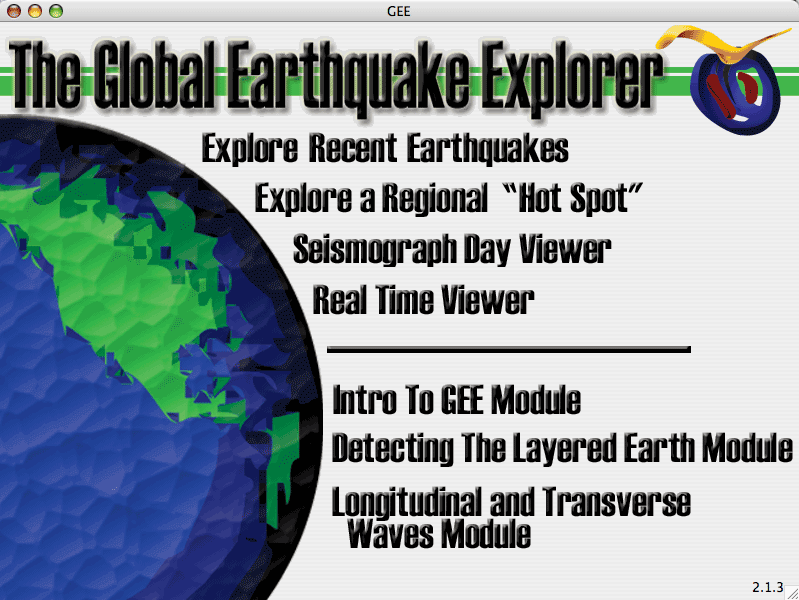
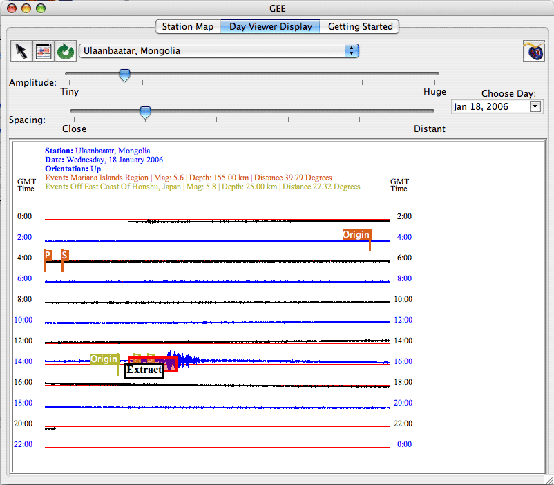
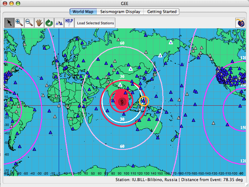
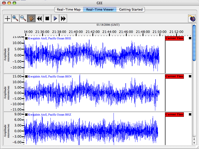
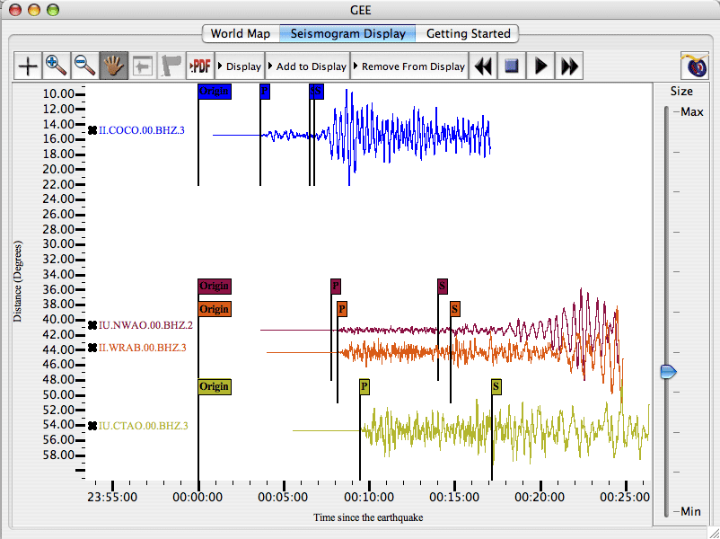
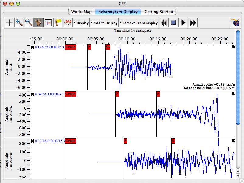
GEE is an education and outreach tool for seismology that aims to make it easy for non-seismologists to retrieve, display and analyze seismic data. It is intended for use in a classroom setting as a supplement to textbook material, which often lacks real world connections. Novices to the world of seismology can use GEE to explore earthquakes they’ve seen in the headlines, keep track of a recording station in their area, look at real-time seismic data, and more!
GEE is comprised of configurable learning “modules” that can be used to convey specific seismological concepts such as wave properties, the structure of the earth, and the differences between P and S waves. The modules provided with GEE are the ones developed for use by the South Carolina Earth Physics Project.
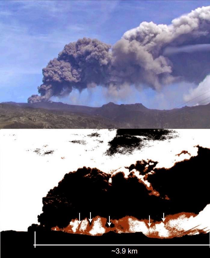
Figure 1 from Manzella et al.: Original and processed snapshot of the video of the Eyjafjallajökull (Iceland) plume as observed on May 4, 2010. White arrows indicate finger positions. Credit: Manzella et al. and Geology
Volcanic ash poses a significant hazard for areas close to volcanoes and for aviation. For example, the 2010 eruption of Eyjafjallajökull, Iceland, clearly demonstrated that even small-to-moderate explosive eruptions, in particular if long-lasting, can paralyze entire sectors of societies, with significant, global-level, economic impacts. In this open-access Geology article, Irene Manzella and colleagues present the first quantitative description of the dynamics of gravitational instabilities and particle aggregation based on the 4 May 2010 eruption.
Their analysis also reveals some important shortcomings in the Volcanic Ash Transport and Dispersal Models (VATDMs) typically used to forecast the dispersal of volcanic ash. In particular, specific processes exist that challenge the view of sedimentation of fine particles from volcanic plumes and that are currently poorly understood: particle aggregation and gravitational instabilities. These appear as particle-rich “fingers” descending from the base of volcanic clouds and have commonly been observed during volcanic explosive eruptions.
Based on direct observations of the 2010 Eyjafjallajökull plume, on the correlation with the associated fallout deposit, and on dedicated laboratory analogue experiments, Irene Manzella and colleagues show how fine ash in these particle-rich fingers settles faster than individual particles and that aggregation and gravitational instabilities are closely related. Both phenomena can significantly contribute to reducing fine-ash lifetime in the atmosphere and, therefore, it is crucial to include them in VATDMs in order to provide accurate forecasting of ash dispersal and sedimentation.
Reference:
I. Manzella, C. Bonadonna, J. C. Phillips, H. Monnard. The role of gravitational instabilities in deposition of volcanic ash. Geology, 2015; DOI: 10.1130/G36252.1
An international research team led by the High Council for Scientific Research (CSIC in its Spanish acronym) and with the participation of the University of Granada, has found that there is a direct relation between the changes in the earth’s orbit and the stability of the Eastern ice cap of Antarctica, more specifically, on the continental fringe of Wilkes Land (East Antarctica). 29 scientists from 12 different countries participated in this study, which has been published in the journal Nature Geosciences.
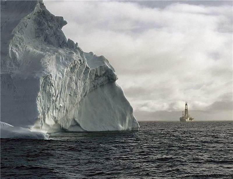
This study is based upon the analysis of seabed sediments which were transported by icebergs around 2.2 to 4.3 million years ago, and which have been collected during an expedition by the Integrated Ocean Drilling Program.
The data obtained reveal that natural climatic processes can increase the response of polar ice caps to minor changes in energy caused by modifications in earth’s orbit. The sea level can either decrease or increase by as much as dozens of meters. This study shows that 2.5 million years ago, when the concentration of carbon dioxide in the atmosphere was similar to the current one, the thawing of the eastern Antarctic ice cap was a generalized process.
“This study helps solve the mystery of how the Earth’s orbit around the Sun contributes to the stability of ice caps,” according to Carlota Escutia, a researcher at the Andalusian Institute of Earth Sciences (a CSIC-UGR joint institution), which has led the expedition.
Greenhouse effect gases
“The emission of greenhouse effect gases has, nevertheless, a much larger energy impact than that provided by any changes in the earth’s orbit,” according to Escutia.
The analysis of sediments shows that the stability of the largest ice cap on earth is influenced by the presence of sea ice in the oceans that surround Antarctica. This sea ice is a layer of frozen seawater that creates a protective shield around the continent and the Antarctic ice caps, and it is sensitive to the warming up of oceans generated as a result of the increase in greenhouse effect gasses. “The disappearance of this sea ice can result in the melting of the ice caps and in the increase of sea level by several meters,” adds Escutia.
Millions of years ago, under conditions of high concentration of carbon dioxide — as is also the case now — and ocean temperatures slightly higher than those currently registered, the oceans surrounding Antarctica could no longer sustain the sea ice. Escutia points out that “the disappearance of this protective shield allowed oceanic currents pushed by the winds to penetrate down to the base of the ice caps, provoking their thaw.”
This study speculates with a potentially generalized thaw of Antarctica’s Eastern ice cap in the future if we fail to reduce the levels of carbon dioxide in the atmosphere.
Reference:
M. O. Patterson, R. McKay, T. Naish, C. Escutia, F. J. Jimenez-Espejo, M. E. Raymo, S. R. Meyers, L. Tauxe, H. Brinkhuis, A. Klaus, A. Fehr, J. A. P. Bendle, P. K. Bijl, S. M. Bohaty, S. A. Carr, R. B. Dunbar, J. A. Flores, J. J. Gonzalez, T. G. Hayden, M. Iwai, K. Katsuki, G. S. Kong, M. Nakai, M. P. Olney, S. Passchier, S. F. Pekar, J. Pross, C. R. Riesselman, U. Röhl, T. Sakai, P. K. Shrivastava, C. E. Stickley, S. Sugasaki, S. Tuo, T. van de Flierdt, K. Welsh, T. Williams, M. Yamane. Orbital forcing of the East Antarctic ice sheet during the Pliocene and Early Pleistocene. Nature Geoscience, 2014; 7 (11): 841 DOI: 10.1038/NGEO2273
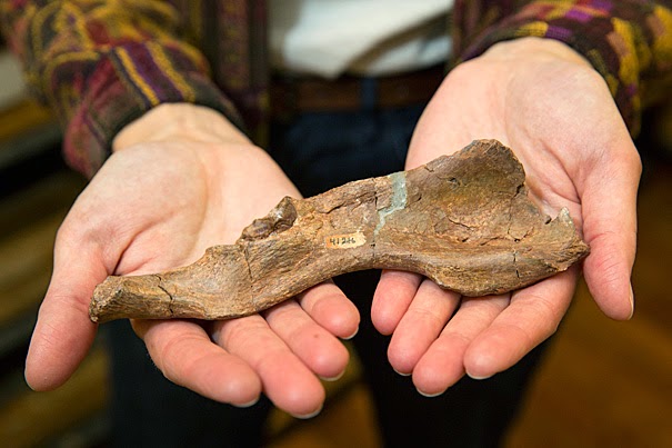
The fossilized hipbone of an ape called Sivapithecus is raising a host of new questions about whether the upright body plan of apes may have evolved multiple times. “What we do know is that the evolution of the orthograde body plan in apes is not a simple story,” noted Harvard’s Michèle Morgan, co-author of the paper. Jon Chase/Harvard Staff Photographer
For decades, scientists have recognized the upright posture exhibited by chimpanzees, gorillas, and humans as a key feature separating the “great apes” from other primates, but a host of questions about the evolution of that posture—particularly how and when it emerged—have long gone unanswered.
For more than a century, the belief was that the posture, known as the orthograde body plan, evolved only once, as part of a suite of features, including broad torsos and mobile forelimbs, in an early ancestor of modern apes.
But a fossilized hipbone of an ape called Sivapithecus is challenging that belief.
The bone, about 6 inches long, is described in a paper in the Proceedings of the National Academy of Sciences (PNAS) co-authored by Michèle Morgan, museum curator of osteology and paleoanthropology at Harvard’s Peabody Museum of Archaeology and Ethnology, and colleagues including Kristi Lewton, Erik Otárola-Castillo, John Barry, Jay Kelley, Lawrence Flynn, and David Pilbeam. The finding has raised a host of new questions about whether that upright body plan may have evolved multiple times.
“We always thought if we found this body part, that it would show some of the features we find in the living great apes,” Morgan said. “To find something like this was surprising.”
Where modern apes have large, broad chests, Sivapithecus is believed to have had a relatively narrow, monkey-like torso, but facial features that closely resemble modern orangutans. That mixture, showing some ape- and monkey-like features, has left researchers scratching their heads about the arrangement of the primate tree, and raises questions about how the stereotypically ape-like body plan evolved.
“Today, all the living great apes—gorillas, orangutans, chimps—have very broad torsos … and people had commonly thought that this torso shape was shared among all the great apes, meaning it must have evolved in a common ancestor,” Morgan said.
“We initially believed that Sivapithecus, with a narrow torso, was on the orangutan line, but if that is the case, then the great ape body shape would have had to evolve at least twice,” she added. “There are a lot of questions that this fossil raises, and we don’t have good answers for them yet. What we do know is that the evolution of the orthograde body plan in apes is not a simple story.”
What Sivapithecus may ultimately demonstrate, said Flynn, assistant director of the American School of Prehistoric Research at the Peabody Museum, is that evolution doesn’t occur in a straight line, but happens as a mosaic across many species.
“What this speaks to is a rich tree with a lot of branches,” Flynn said. “There are not just one or two branches that reach back into the Miocene (epoch). It’s a very rich and complex tree.
“I think we sometimes take the easy route of trying to understand these fossils based on creatures we find today,” Flynn said. “But what we’re finding out time and again is these 10- or 12- or 15-million-year-old creatures were their own entities. Today is not always a very good model for the past.”
To fully understand where Sivapithecus belongs in the evolutionary tree of apes, Flynn said, more fossils must be found, and additional research must be conducted.
“It’s a very easy thing for people to ask, why do we need to go find more fossils; don’t we already know everything? The answer is no,” he said. “We’re only just beginning to understand what we don’t know. And as we learn more, there are more interesting and exciting questions we can ask, and hopefully we can answer.”
Note : The above story is based on materials provided by Harvard University. The original article was written by Peter Reuell.
Acoustic-gravity waves—a special type of sound wave that can cut through the deep ocean at the speed of sound—can be generated by underwater earthquakes, explosions, and landslides, as well as by surface waves and meteorites. A single one of these waves can stretch tens or hundreds of kilometers, and travel at depths of hundreds or thousands of meters below the ocean surface, transferring energy from the upper surface to the seafloor, and across the oceans. Acoustic-gravity waves often precede a tsunami or rogue wave—either of which can be devastating.
Now a new study by an MIT researcher suggests that these immense deep-ocean waves can rapidly transport millions of cubic meters of water, carrying salts, carbons, and other nutrients around the globe in a matter of hours.
Usama Kadri, a postdoc in MIT’s Department of Mechanical Engineering, tracked the theoretical movement of fluid caught up in an acoustic-gravity wave at various depths in the ocean, ranging from hundreds to thousands of meters below the surface. Based on his calculations, Kadri found that acoustic-gravity waves can push parcels significant distances, depending on their depth.
“Deep-water transport is so vital—not only to local marine ecosystems, but to our global ecosystem and environment—that a cut in such transport will ultimately result in the death of marine life, create regions of extreme water temperatures, and dramatically affect our climate,” says Kadri, who has published his results in the Journal of Geophysical Research: Oceans. “To sustain a healthier global ecosystem and environment, there is a need to increase awareness of acoustic-gravity waves and deep-water transport.”
Kadri adds that such awareness may help scientists devise early-warning systems for seaside communities and offshore facilities vulnerable to tsunamis or rogue waves—monster waves that can come on suddenly, with potentially devastating effects.
“Since acoustic-gravity waves are so much faster than tsunamis or rogue waves, successful recordings of … acoustic-gravity waves would enhance current warning systems dramatically, and improve detection by minutes to hours depending on the source location,” Kadri says, “either of which is sufficient to [save] many lives.”
Acoustics and gravity
A gravity wave is generated in a fluid or at the interface between fluids, and is governed by gravity. A common example is an ocean surface wave.
Acoustic waves, by contrast, propagate through longitudinal compression. For example, sound travels by vibrating and pushing against a fluid medium. Unlike in gravity waves, compressibility dominates acoustic waves, while the effect of gravity is negligible.
For those reasons, Kadri says, scientists have generally studied either sound waves in the ocean from a purely acoustic perspective, or surface waves in an incompressible ocean.
Drifting with the wave
Kadri modeled the behavior of acoustic-gravity waves in the deep ocean by first considering the propagation of waves in an ideal, compressible ocean, where water volume changes slightly in response to pressure changes. In a two-dimensional model, he calculated the movement of fluid caused by a traveling acoustic-gravity wave at various depths in the ocean.
Kadri’s equations showed that acoustic-gravity waves may propagate throughout the ocean, up to thousands of meters deep, even traveling along the seafloor. He then looked into whether acoustic-gravity waves may cause water to drift long distances, or if they simply recirculate them back to their original location.
Kadri worked the equation out for acoustic-gravity waves at various depths in the deep ocean, and found that these waves can transport water at a velocity of a few centimeters per second. Such waves, Kadri estimates, can therefore transport millions of cubic meters of deep water per second.
According to these results, acoustic-gravity waves may be “major players,” Kadri says, in transporting water and producing currents in the deep ocean. Such waves may be instrumental in carrying plankton, algae, and bacteria across the oceans, as well as in delivering essential nutrients to sedentary marine organisms.
Knowing the properties of acoustic-gravity waves may also help researchers develop early-warning systems for potentially devastating ocean events, such as tsunamis and rogue waves. Toward that end, Kadri is continuing his work to develop predictive computations that can analyze acoustic signals for fast-traveling acoustic-gravity waves—a precursor to tsunamis.
Jerry Smith, a research oceanographer at the University of California at San Diego, says a striking contribution from Kadri’s research is the finding that surface waves have an effect on deep-ocean waves.
“The most significant finding in this particular paper is the contribution to deep-ocean transport,” says Smith, who was not involved in the research. “This has not been appreciated before. Since these acoustic-gravity waves can be generated by nonlinear interactions of ordinary wind-waves, the contribution to deep transport could be ubiquitous.”
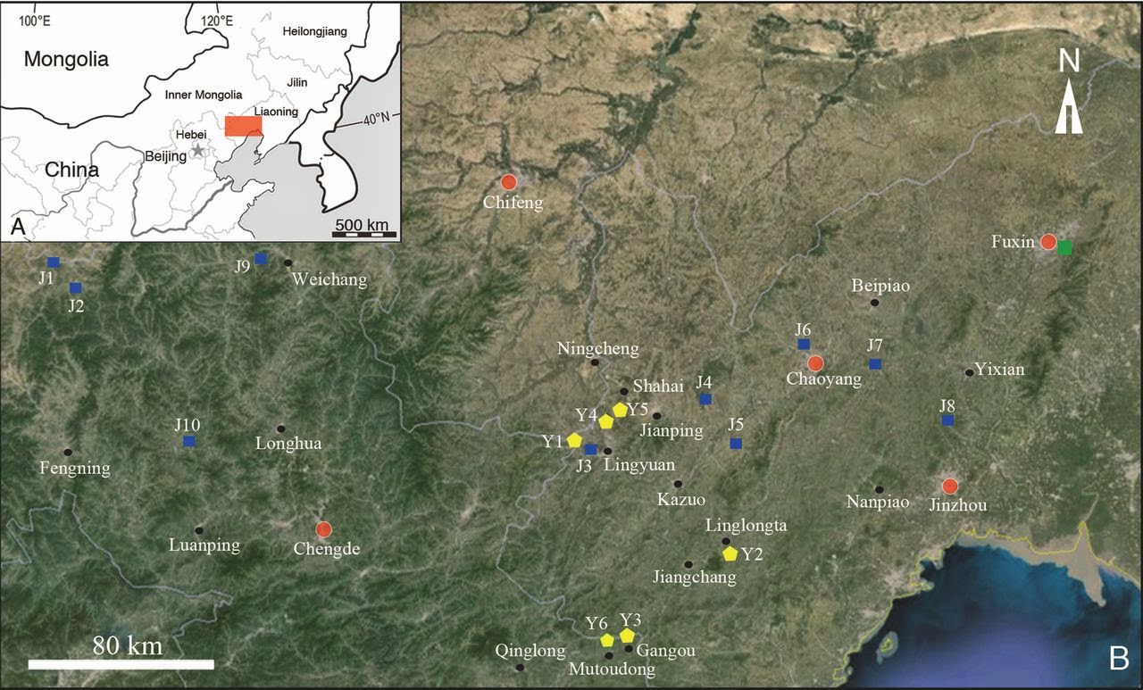
Geographic map of main fossil localities that yield the Yanliao (Daohugou), Jehol and Fuxin biotas in northeast China. Credit: Science China Press
The most exciting findings covering Mesozoic mammals over the last two decades have come from the Jurassic and Cretaceous periods of China. Remarkably preserved fossils across nearly all major groups of Mesozoic mammals have provided a great amount of information about their morphology and biology. A researcher at the American Museum of Natural History reviews these discoveries and outlines potential future research efforts in the study of mammalian evolution.
It is generally accepted that the tree of life for mammals was rooted in the Mesozoic, but the specific time for the origin of mammals remains an issue of debate. This is partly because Mesozoic mammals are commonly known by fragmentary material, mostly dentitions, that restrained the search for the biology and evolution of our earliest ancestors.
During the last two decades, many Mesozoic mammals have been reported from all over the world. Notable among them are those from the southern continents, which have significantly enriched understanding of the morphology, diversity, geographic distribution and evolution of Mesozoic mammals. The most remarkable discoveries, however, have come from the Jurassic and Cretaceous periods of China; approximately 50 species, with most represented by superbly preserved skeletal specimens, have been reported. These discoveries have cast new light on some important issues in the study of Mesozoic mammals, such as the diversity and disparity, the mammalian affinity of “haramiyidans”, the divergence time of mammals and evolution of the mammalian middle ear.
Many issues regarding these findings are still being debated, and their resolution might depend on new discoveries and analyses. In a new study, Jin Meng, a scientist at the American Museum of Natural History in New York, reviews a spectrum of discoveries made surrounding the Mesozoic mammals of China. Meng, who is also based at the prestigious Institute of Vertebrate Paleontology and Paleoanthropology in Beijing, outlines these findings in an article titled “Mesozoic mammals of China: implications for phylogeny and early evolution of mammals” published in the Beijing-based journal National Science Review.
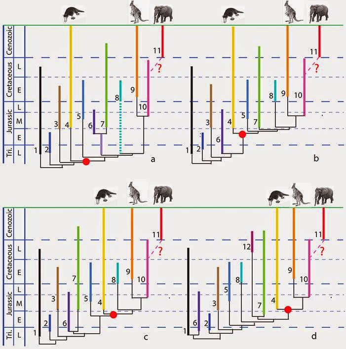
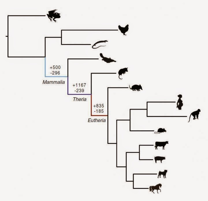
The study reviews most known Mesozoic mammals from China, which can be divided into several assemblages according to their geographic and temporal distribution; it also covers different evolutionary stages that are largely consistent with the global pattern of mammalian evolution. Also reviewed are varying hypotheses on the divergent times and phylogenetic relationships of Mammalia and its subgroups (Fig. 1), which in turn significantly affect interpretation of character evolution in early mammals.
The divergence time of Mammalia is directly associated with how the phylogeny of mammals is reconstructed, particularly with the phylogenetic placement of ‘haramiyidans’, a long-time puzzle in paleo-mammalian taxonomy and phylogeny. In light of the discoveries of several species that formed the clade Euharamiyida, the mammalian affinity of ‘haramiyidans’ was strongly supported by dental, cranial and postcranial features from these euharamiyidans. In the preferred phylogeny (Fig. 1a), Allotheria (‘haramiyidans’ and multituberculates) are placed within Mammalia, which best incorporated available evidence of morphology, temporal distributions and most phylogenetic analyses of known Mesozoic mammals and kept character parallelisms at the minimum between ‘haramiyidans’ and multituberculates, as well as between allotherians and other mammals. This hypothesis suggests that mammals originated in an explosive fashion during the Late Triassic because members of allotherians were found in beds of the Late Triassic.
As an example of character evolution of mammals, the study outlines the evolution of the mammalian middle ear, a classic issue of gradual evolution in vertebrates. All extant mammals have three middle ear ossicles: the malleus, incus and stapes. In addition, there is the ectotympanic that holds the eardrum. It has been known from developmental studies that the malleus is a composite element equivalent to the articular and prearticular, the incus is equivalent to the quadrate and the ectotympanic is equivalent to the angular bone. It is also known from the fossil record that during the evolution of mammals, the postdentary bones in the lower jaw of non-mammalian cynodonts were gradually reduced in size and eventually migrated to the middle ear. Research on eutriconodontans and ‘symmetrodontans’ from the Jehol Biota has provided evidence on the transitional mammalian middle ear (TMME), an immediate form between the mandibular ear and the definitive mammalian middle ear (DMME). The mandibular middle ear is a complex in which the ear bones are small but still attached to the tooth-bearing dentary bone so that these small bones have a dual function: mastication and hearing, as seen in Morganucodon. In the DMME the ear ossicles were completely detached from the dentary bone and migrated to the basal cranial region where they function exclusively for hearing. The TMME demonstrates that during the transition from the mandibular middle ear to the DMME, the postdentary bones were detached from the dentary but were not yet securely supported by cranial structures; instead they were anteriorly in articulation with an ossified Meckel’s cartilage whose anterior portion was loosely lodged in a groove on the medial side of the dentary bone. The embryonic condition of the middle ear in living mammals displays a similar morphology to the TMME and probably recapitulates the evolutionary stage of the mammalian middle ear.
Jin Meng also proposes a hypothesis on the evolution of the allotherians tooth pattern to show the potential for future studies based on the Mesozoic mammals discovered in China. The basic allotherian tooth pattern consists of two rows of multiple cusps in the upper and lower molars and is capable of a posterior, not transverse, chewing motion. This tooth pattern differs from those of other mammals that evolved from a ‘triconodont’-like tooth pattern to a tribosphenic tooth pattern. How the allotherian tooth pattern evolved has remained an enigma in the study of mammalian evolution. It is puzzling because wherever allotherians are placed in the phylogeny, either within or outside Mammalia, it is equally difficult to derive the allotherian tooth pattern from any known mammals or their close kin. Given the preferred phylogeny (Fig. 1a), which suggests that allotherians were derived from a Haramiyavia-like ancestor, and the occlusal pattern revealed by the euharamiyidans, it is proposed that the primitive allotherian tooth pattern, as represented by Haramiyavia, could have evolved from a ‘triconodont’-like tooth pattern and then gave rise to those of euharamiyidans and multituberculates, respectively.
Reference:
Jin Meng. “Mesozoic mammals of China: implications for phylogeny and early evolution of mammals.” National Science Review, doi: 10.1093/nsr/nwu070
Note : The above story is based on materials provided by Science China Press.
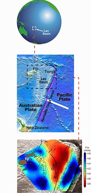
The Lau Basin, in the South Pacific (top), is a V-shaped basin created by the subduction of the Pacific Plate at the Tonga Trench (the purple line in the central image). A seismic image (bottom) of part of the basin at a depth of 50 kilometers (31 miles) shows magma pooling to the north beneath areas that are unrifted (dark red) and provide no egress but little magma (pale yellow) along the southern end of the Eastern Lau Spreading Center, or ELSC, even though this area is intensely volcanic. Credit: Wei/Wiens
It was a bit like making a CT scan of a patient’s head and finding he had very little brain or making a PET scan of a dead fish and seeing hot spots of oxygen consumption. Scientists making seismic images of the mantle beneath a famous geological site saw the least magma where they expected to see the most.
What was going on? Was it an artifact of their technique or the revelation of something real but not yet understood?
In the online Feb. 2 issue of Nature, a team of scientists, led by S. Shawn Wei and Douglas Wiens of Washington University in St. Louis, published a three-dimensional seismic image of mantle beneath the Lau Basin in the South Pacific that had an intriguing anomaly.
The basin is an ideal location for studying the role of water in volcanic and tectonic processes. Because the basin is widening, it has many spreading centers, or deep cracks through which magma rises to the surface. And because it is shaped like a V, these centers lie at varying distances from the Tonga Trench, where water is copiously injected into Earth’s interior.
The scientists knew that the chemistry of the magma erupted through the spreading centers varies with their distance from the trench. Those to the north, toward the opening of the V, erupt a drier magma than those to the south, near the point of the V, where the magma has more water and chemical elements associated with water. Because water lowers the melting temperature of rock, spreading centers to the north also produce less magma than those to the south.
Before they constructed images from their seismic data, the scientists expected the pattern in the mantle to match that on the surface. In particular they expected to find molten rock pooled to the south, where the water content in the mantle is highest. Instead the seismic images indicated less melt in the south than in the north.
They were flummoxed. After considerable debate, they concluded they were seeing something real. Water, they suggest, increases melting but makes the melt less viscous, speeding its transport to the surface, rather like mixing water with honey makes it flow quicker. Because water-laden magma flushes out so quickly, there is less of it in the mantle at any given moment even though more is being produced over time.
The finding brings scientists one step closer to understanding how the Earth’s water cycle affects nearly everything on the planet — not just the clouds and rivers above the surface, but also processes that take place in silence and darkness in the plutonic depths.
Stretched thin and ripping
The Lau Basin, which lies between the island archipelagos of Tonga and Fiji, was created by the collision of the giant slab of the Pacific Ocean’s floor colliding with the Australian plate. The older, thus colder and denser, Pacific plate nosed under the Australian plate and sank into the depths along the Tonga Trench, also called the Horizon Deep.
Water given off by the wet slab lowered the melting point of the rock above, causing magma to erupt and form a volcanic arc, called the Tonga-Kermadec ridge.
About 4 to 6 million years ago, the Pacific slab started to pull away from the Australian slab, dragging material from the mantle beneath it. The Australian plate’s margin stretched, splitting the ridge, creating the basin and, over time, rifiting the floor of the basin. Magma upwelling through these rifts created new spreading centers.
“Leave it long enough,” said Wei, a McDonnell Scholar and doctoral student in earth and planetary science in Arts & Sciences, “and the basin will probably form a new ocean.”
“The Tonga subduction zone is famous in seismology,” Wiens said, “because two-thirds of the world’s deep earthquakes happen there and subduction is faster there than anywhere else in the world. In the northern part of this area the slab is sinking at about 24 centimeters (9 inches) a year, or nearly a meter every four years. That’s four times faster than the San Andreas fault is moving.”
The magma that wasn’t there
The images of the mantle published in Nature are based on the rumblings of 200 earthquakes picked up by 50 ocean-bottom seismographs deployed in the Lau Basin in 2009 and 2010 and 17 seismographs installed on the islands of Tonga and Fiji.
The 2009-2010 campaign, led by Wiens, PhD, professor of earth and planetary sciences in Arts & Sciences, was one the largest long-term deployments of ocean-bottom seismographs ever undertaken.
When the scientists looked carefully at the southern part of the images created from their seismograph recordings, they were mystified by what they saw — or rather didn’t see. In their color-coded images, the area along the southern end of the spreading center in the tip of the basin, called the ELSC, should have been deep red.
Instead it registered pale yellow or green, as though it held little magma. “It was the reverse of our expectation,” Wei said.
To make these images, the scientists calculated the departure of the seismic velocities from reference values, Wei explained. “If the velocities are much lower than normal we attribute that to the presence of molten rock,” he said. “The lower the velocity, the more magma.”
Because water lowers melting temperatures, the scientists expected to see the lowest velocities and the most magma to the south, where the water content is highest.
Instead the velocities in the north were much lower than those in the south, signaling less magma in the south. This was all the more mystifying because the southern ELSC is intensely volcanic.
If the volcanoes were spewing magma, why wasn’t it showing up in the seismic images?
After considerable debate, the scientists concluded that water from the slab must make melt transport more efficient as well as lowering melting temperatures.
“Where there’s very little water, the system is not moving the magma through very efficiently,” Wiens said. “So where we see a lot of magma pooled in the north, that doesn’t necessarily mean there’s a lot of melting there, just that the movement of the magma is slow.”
“Conversely, where there’s water, the magma is quickly and efficiently transported to the surface. So where we see little magma in the south, there is just as much melting going on, but the magma is moving through so fast that at any one moment we see less of it in the rock,” Wiens said.
“The only way to explain the distribution of magma is to take account of the effect of water on the transport of magma,” Wei said. “We think water makes the magma significantly less viscous, and that’s why transport is more efficient.”
“This is the first study to highlight the effect of water on the efficiency of magma extraction and the speed of magma transport,” Wiens said.
Wei plans to continue following the water. “A recent paper in Nature described evidence that water is carried down to 410 kilometers (250 miles). I’d like to look deeper,” he said.
Video:
Reference:
S. Shawn Wei, Douglas A. Wiens, Yang Zha, Terry Plank, Spahr C. Webb, Donna K. Blackman, Robert A. Dunn, James A. Conder. Seismic evidence of effects of water on melt transport in the Lau back-arc mantle. Nature, 2015; DOI: 10.1038/nature14113
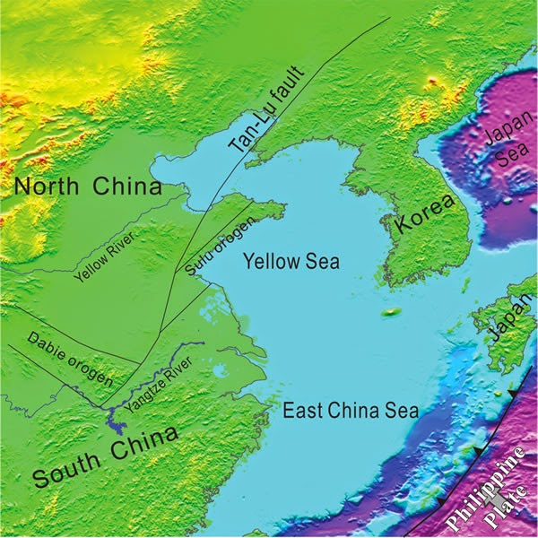
Color-shaded relief map with simplified tectonic units of eastern Asia. Since the Late Cretaceous, lithosphere extension was induced by the subduction of the western Pacific or Philippine plate. The Dabie and Sulu orogens contain the largest ultrahigh-pressure metamorphic belt in the world as a result of the convergence between the North and South China blocks during the Late Paleozoic–Triassic. Credit: Copyright Tian and Santosh, GSA Today Feb. 2015
Seismic investigations from the Qinling-Dabie-Sulu orogenic belt in eastern China suggest that this region was affected by extreme mantle perturbation and crust-mantle interaction during the Mesozoic era. The Qinling-Dabie-Sulu orogenic belt formed through the collision between the North and South China blocks, which produced large-scale destruction of the cratonic lithosphere, accompanied by widespread magmatism and metallogeny.
Global mantle convection significantly impacts processes at the surface of Earth and can be used to gain insights on plate driving forces, lithospheric deformation, and the thermal and compositional structure of the mantle. Upper-mantle seismic anisotropy is widely employed to study both present and past deformation processes at lithospheric and asthenospheric depths.
The majority of seismic data from stations located near Qinling-Dabie-Sulu orogenic belt show anisotropy with an E-W- or ENE-WSW-trending fast polarization direction, parallel to the southern edge of the North China block. This suggests compressional deformation in the lithosphere due to the collision between the North and South China blocks.
Although the deep root of the craton was largely destroyed by cratonic reactivation in the late Mesozoic, these results suggest that the “fossilized” anisotropic signature is still preserved in the remnant lithosphere beneath eastern China.
Reference:
Xiaobo Tian, M. Santosh. Fossilized lithospheric deformation revealed by teleseismic shear wave splitting in eastern China. GSA Today, 2015; 4 DOI: 10.1130/GSATG220A.1
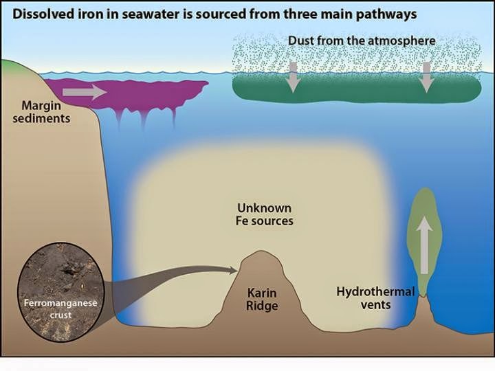
While many areas of the ocean are rich in other nutrients, they often lack iron — a critical element for marine life. Dissolved iron in seawater can originate from three main sources: Dust from the atmosphere, sediment dissolution along continental margins, and fluids from hydrothermal vents. Credit: Jack Cook, Woods Hole Oceanographic Institution
A new study led by scientists at the Woods Hole Oceanographic Institution (WHOI) points to the deep ocean as a major source of dissolved iron in the central Pacific Ocean. This finding highlights the vital role ocean mixing plays in determining whether deep sources of iron reach the surface-dwelling life that need it to survive.
“Our study is a long-term view–over the past 76 million years–of where iron has been coming from in the central Pacific,” says Tristan Horner, a postdoctoral fellow in the Marine Chemistry and Geochemistry Department at WHOI and lead author of the paper to be published February 3, 2015, in Proceedings of the National Academy of Sciences.
While many areas of the ocean are rich in other nutrients, they often lack iron–a critical element for marine life. Iron is particularly important for the growth of phytoplankton, which are tiny plant-like organisms that form the base of the ocean food chain and play an important role in Earth’s climate.
In addition to producing about half of the planet’s oxygen, phytoplankton live at the ocean’s surface and act as sponges of carbon dioxide–a heat-trapping gas. Through photosynthesis, phytoplankton take carbon from the air into their bodies. When they die or are eaten, much of the carbon sinks to the deep ocean, where it cannot re-enter the atmosphere.
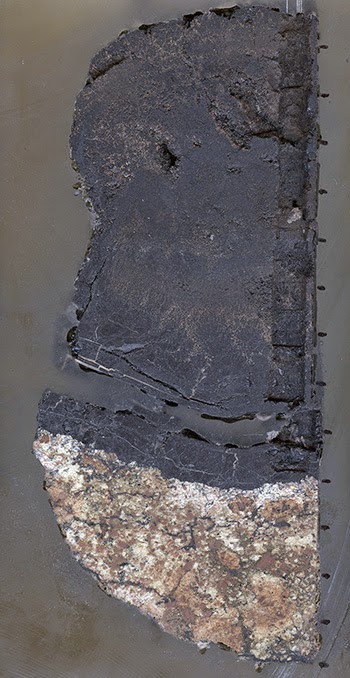
Using a mass spectromemter, the ferromanganese crust sample (Tristan Horner, Woods Hole Oceanographic Institution )
“In basic terms, iron is so important because it helps control climate,” says Sune Nielsen, a WHOI geologist and coauthor. “We need to understand where iron in the ocean is coming from in order to truly understand the role of iron in the marine carbon cycle.”
The scientific community has long thought that the vast majority of the ocean’s iron comes from atmospheric dust, with smaller inputs from dissolved sediment along continental margins, and fluids from hydrothermal vents, which are mineral-rich hot springs on the seafloor, miles below the surface.
Iron is readily soluble in low oxygen regions at hydrothermal vent sites and along continental margins, but it was believed the iron remained in these localized spots and didn’t contribute much to the overall iron content of the ocean. “According to conventional wisdom, as soon as these iron-rich fluids hit seawater with high oxygen concentrations, the iron would just dump out and never really go anywhere,” explains Nielsen.
However, Horner says, “That is not the case, at least in the central Pacific Ocean. We found that much of the dissolved iron in that region originated from hydrothermal vents and sediments thousands of meters below the sea surface. And we found that the iron from these deep sources can be transported long distances.”
To conduct their research, the researchers analyzed a marine sediment, called a ferromanganese crust, taken from a spot far from any hydrothermal vent sites in the central Pacific Ocean. The sample was collected from the flank of the Karin Ridge, a seamount located in the central Pacific, in the 1980s by coauthor Jim Hein of the U.S. Geological Survey (USGS) in Santa Cruz, from a dredge along the seafloor.
The team used a mass spectrometer to analyze the sample for long-term changes in seawater isotopic chemistry recorded in the growth layers of the ferromanganese crust, which forms very slowly. Drilling cross sections in the sample allowed scientists to look through “sections of time” to analyze variations in the composition of iron isotopes–stable natural isotopes iron-56 and iron-54–in order to track the origins of iron.
“The ratio of iron isotopes vary among the different iron sources–atmospheric dust, hydrothermal vents, and dissolved sediments– and are actually quite distinct, like fingerprints. We were able to measure those ratios in the growth layers of our sample, which tells us about where the iron came from and how the different iron sources have waxed and waned over time,” Horner says.
“This study is exciting in that it applies some of the recently developed metal isotope capabilities to parse the different sources of scarce iron in seawater going back through time, and builds on the emerging story about the importance of hydrothermal vents to the inventory of iron in the sea,” adds Mak Saito, a biogeochemist at WHOI and one of the coauthors of the study.
The researchers hope to use this technique to look at iron sources in other parts of the ocean. Future studies could help answer lingering questions about global iron budgets, the influence of iron on climate, and how hydrothermal vents affect the ocean as a whole. Reference:
Tristan J. Horner, Helen M. Williams, James R. Hein, Mak A. Saito, Kevin W. Burton, Alex N. Halliday, Sune G. Nielsen. Persistence of deeply sourced iron in the Pacific Ocean. Proceedings of the National Academy of Sciences, 2015; 201420188 DOI: 10.1073/pnas.1420188112
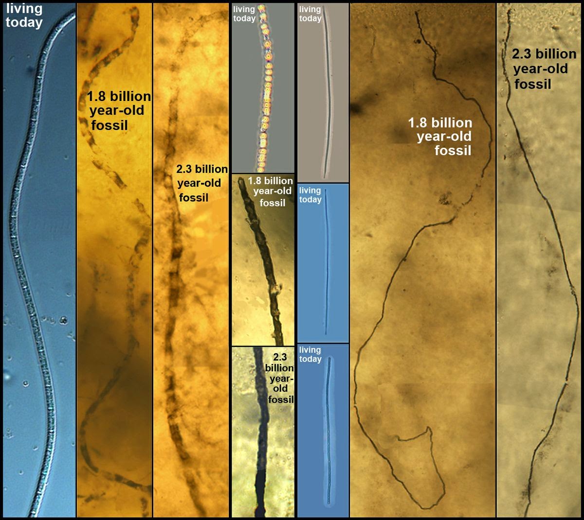
Deep-sea microorganisms are unchanged over more than 2 billion years. Credit : UCLA Center for the Study of Evolution and the Origin of Life
An international team of scientists has discovered the greatest absence of evolution ever reported — a type of deep-sea microorganism that appears not to have evolved over more than 2 billion years. But the researchers say that the organisms’ lack of evolution actually supports Charles Darwin’s theory of evolution.
The findings are published online today by the Proceedings of the National Academy of Sciences.
The scientists examined sulfur bacteria, microorganisms that are too small to see with the unaided eye, that are 1.8 billion years old and were preserved in rocks from Western Australia’s coastal waters. Using cutting-edge technology, they found that the bacteria look the same as bacteria of the same region from 2.3 billion years ago — and that both sets of ancient bacteria are indistinguishable from modern sulfur bacteria found in mud off of the coast of Chile.
“It seems astounding that life has not evolved for more than 2 billion years — nearly half the history of the Earth,” said J. William Schopf, a UCLA professor of earth, planetary and space sciences in the UCLA College who was the study’s lead author. “Given that evolution is a fact, this lack of evolution needs to be explained.”
Charles Darwin’s writings on evolution focused much more on species that had changed over time than on those that hadn’t. So how do scientists explain a species living for so long without evolving?
“The rule of biology is not to evolve unless the physical or biological environment changes, which is consistent with Darwin,” said Schopf, who also is director of UCLA’s Center for the Study of Evolution and the Origin of Life. The environment in which these microorganisms live has remained essentially unchanged for 3 billion years, he said.
A section of a 1.8 billion-year-old fossil-bearing rock. Credit : UCLA Center for the Study of Evolution and the Origin of Life
“These microorganisms are well-adapted to their simple, very stable physical and biological environment,” he said. “If they were in an environment that did not change but they nevertheless evolved, that would have shown that our understanding of Darwinian evolution was seriously flawed.”
Schopf said the findings therefore provide further scientific proof for Darwin’s work. “It fits perfectly with his ideas,” he said.
The fossils Schopf analyzed date back to a substantial rise in Earth’s oxygen levels known as the Great Oxidation Event, which scientists believe occurred between 2.2 billion and 2.4 billion years ago. The event also produced a dramatic increase in sulfate and nitrate — the only nutrients the microorganisms would have needed to survive in their seawater mud environment — which the scientists say enabled the bacteria to thrive and multiply.
Schopf used several techniques to analyze the fossils, including Raman spectroscopy — which enables scientists to look inside rocks to determine their composition and chemistry — and confocal laser scanning microscopy — which renders fossils in 3-D. He pioneered the use of both techniques for analyzing microscopic fossils preserved inside ancient rocks.
Co-authors of the PNAS research were Anatoliy Kudryavtsev, a senior scientist at UCLA’s Center for the Study of Evolution and the Origin of Life, and scientists from the University of Wisconsin, NASA’s Jet Propulsion Laboratory, Australia’s University of New South Wales and Chile’s Universidad de Concepción.
Schopf’s research is funded by the NASA Astrobiology Institute.
Reference :
Sulfur-cycling fossil bacteria from the 1.8-Ga Duck Creek Formation provide promising evidence of evolution’s null hypothesis
Author contributions: J.W.S., K.H.W., and J.W.V. designed research; J.W.S., A.B.K., M.R.W., M.J.V.K., K.H.W., R.K., V.A.G., C.E., and D.T.F. performed research; J.W.S., A.B.K., M.R.W., M.J.V.K., K.H.W., R.K., J.W.V., V.A.G., C.E., and D.T.F. analyzed data; and J.W.S., M.R.W., K.H.W., J.W.V., and V.A.G. wrote the paper. Doi: 10.1073/pnas.1419241112
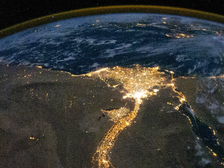
The Nile River and Delta, viewed at night by the Expedition 25 crew on Oct. 28, 2010. Credit: NASA
Planet Earth boasts some very long rivers, all of which have long and honored histories. The Amazon, Mississippi, Euphrates, Yangtze, and Nile have all played huge roles in the rise and evolution of human societies. Rivers like the Danube, Seine, Volga and Thames are intrinsic to the character of some of our most major cities.
But when it comes to the title of which river is longest, the Nile takes top billing. At 6,583 km (4,258 miles) long, and draining in an area of 3,349,000 square kilometers, it is the longest river in the world, and even the longest river in the Solar System. It crosses international boundaries, its water is shared by 11 African nations, and it is responsible for the one of the greatest and longest-lasting civilizations in the world.
Officially, the Nile begins at Lake Victoria – Africa’s largest Great Lake that occupies the border region between Tanzania, Uganda and Kenya – and ends in a large delta and empties into the Mediterranean Sea. However, the great river also has many tributaries, the greatest of which are the Blue Nile and White Nile rivers.
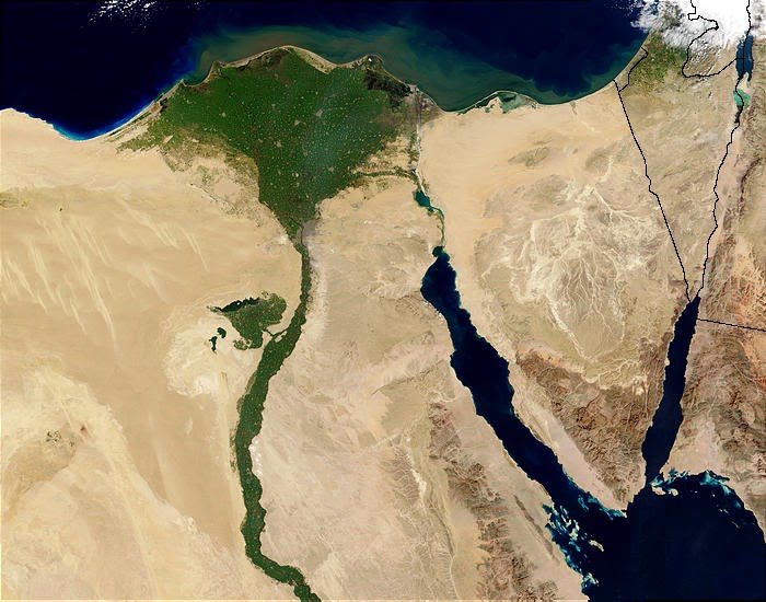
Nile Delta from space by the MODIS sensor on the Terra satellite. Credit: Jacques Descloitres/NASA/GSFC
The White Nile is the source of the majority of the Nile’s water and fertile soil, and originates from Africa’s Great Lakes region of Central Africa (a group that includes Lake Victoria, Edward, Tanganyika, etc.). The Blue Nile starts at Lake Tana in Ethiopia, and flows north-west to where it meets the Nile near Khartoum, Sudan.
The northern section of the Nile flows entirely through the Sudanese Desert to Egypt. Historically speaking, most of the population and cities of these two countries were built along the river valley, a tradition which continues into the modern age. In addition to the capitol cities of Juba, Khartoum, and Cairo, nearly all the cultural and historical sites of Ancient Egypt are to be found along the riverbanks.
The Nile was a much longer river in ancient times. Prior to the Miocene era (ca. 23 to 5 million years ago), Lake Tangnayika drained northwards into the Albert Nile, making the Nile about 1,400 km. That portion of the river became blocked by the bulk of the formation of the Virunga Mountains through volcanic activity.
Between 8000 and 1000 B.C.E., there was also a third tributary called the Yellow Nile that connected the highlands of eastern Chad to the Nile River Valley. Its remains are known as the Wadi Howar, a riverbed that passes through the northern border of Chad and meets the Nile near the southern point of the Great Bend – the region that lies between Khartoum and Aswan in southern Egypt where the river protrudes east and west before traveling north again.
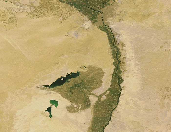
Lake Moeris and Faiyum Oasis, as seen from space, south-west of the Nile Delta and Cairo. Credit: Earth Snapshot
The Nile, as it exists today, is thought to be the fifth river that has flowed from the Ethiopian Highlands. Some form of the Nile is believed to have existed for 25 million years. Satellite images have been used to confirm this, identifying dry watercourses to the west of the Nile that are believed to have been the Eonile.
This “ancestral Nile” is believed to be what flowed in the region during the later Miocene, transporting sedimentary deposits to the Mediterranean Sea. During the late-Miocene Era, the Mediterranean Sea became a closed basin and evaporated to the point of being empty or nearly so. At this point, the Nile cut a new course down to a base level that was several hundred meters below sea level.
This created a very long and deep canyon which was filled with sediment, which at some point raised the riverbed sufficiently for the river to overflow westward into a depression to create Lake Moeris southwest of Cairo. A canyon, now filled by surface drift, represents an ancestral Nile called the Eonile that flowed during the Miocene.
Due to their inability to penetrate the wetlands of South Sudan, the headwaters of the Nile remained unknown to Greek and Roman explorers. Hence, it was not until 1858 when John Speke sighted Lake Victoria that the source of the Nile became known to European historians. He reached its southern shore while traveling with Richard Burton on an expedition to explore central Africa and locate the African Great Lakes.
Believing he had found the source of the Nile, he named the lake after Queen Victoria, the then-monarch of the United Kingdom. Upon learning of this, Burton was outraged that Speke claimed to have found the true source of the Nile and a scientific dispute ensued.
This in turn triggered new waves of exploration that sent David Livingstone into the area. However, he failed by pushing too far to the west where he encountered the Congo River. It was not until the Welsh-American explorer Henry Morton Stanley circumvented Lake Victoria during an expedition that ran from 1874 to 1877 that Speke’s claim to have found the source of the Nile was confirmed.
The Nile became a major transportation route during the European colonial period. Many steamers used the waterway to travel through Egypt and south to the Sudan during the 19th century. With the completion of the Suez Canal and the British takeover of Egypt in the 1870s, steamer navigation of the river became a regular occurrence and continued well into the 1960s and the independence of both nations.
Today, the Nile River remains a central feature to Egypt and the Sudan. Its waters are used by all nations that it passes through for irrigation and farming, and its important to the rise and endurance of civilization in the region cannot be underestimated. In fact, the sheer longevity of Egypt’s many ruling dynasties is often attributed by historians to the periodic flows of sediment and nutrients from Lake Victoria to the delta. Thanks to these flows, it is believed, communities along the Nile River never experienced collapse and disintegration as other cultures did.
The Nile is rivaled only by Amazon, which is also the world’s widest river.
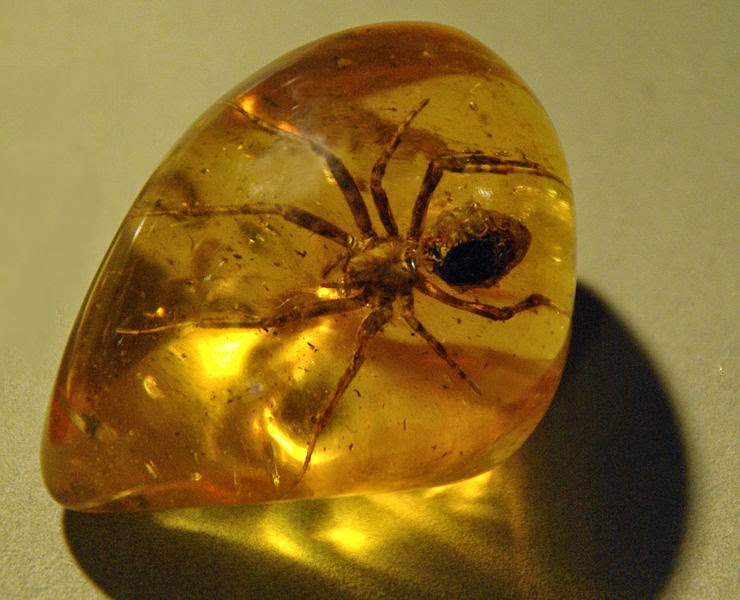
Amber is fossilized tree resin (not sap), which has been appreciated for its color and natural beauty since Neolithic times. Much valued from antiquity to the present as a gemstone, amber is made into a variety of decorative objects. Amber is used as an ingredient in perfumes, as a healing agent in folk medicine, and as jewelry.
There are five classes of amber, defined on the basis of their chemical constituents. Because it originates as a soft, sticky tree resin, amber sometimes contains animal and plant material as inclusions. Amber occurring in coal seams is also called resinite, and the term ambrite is applied to that found specifically within New Zealand coal seams.
What is the History and names of Amber?
The English word amber derives from Arabic ʿanbar عنبر, Middle Latin ambar and Middle French ambre. The word was adopted in Middle English in the 14th century as referring to what is now known as ambergris (ambre gris or “grey amber”), solid waxy substance derived from the sperm whale. In the Romance languages, the sense of the word had come to be extended to Baltic amber (fossil resin) from as early as the late 13th century, at first called white or yellow amber (ambre jaune) for disambiguation, and this meaning was adopted in English by the early 15th century. As the use of ambergris waned, this became the main sense of the word.
The two substances (“yellow amber” and “grey amber”) conceivably became associated or confused because they both were found washed up on beaches. Ambergris is less dense than water and floats, whereas amber is less dense
The classical name for amber was electrum (ἤλεκτρον ēlektron), connected to a term for the “beaming Sun”, ἠλέκτωρ (ēlektōr). According to the myth, when Phaëton son of Helios (the Sun) was killed, his mourning sisters became poplars, and their tears became the origin of elektron, amber.
Amber is discussed by Theophrastus in the 4th century BC, and again by Pytheas (c. 330 BC) whose work “On the Ocean” is lost, but was referenced by Pliny the Elder, according to whose The Natural History (in what is also the earliest known mention of the name Germania):
Pytheas says that the Gutones, a people of Germany, inhabit the shores of an estuary of the Ocean called Mentonomon, their territory extending a distance of six thousand stadia; that, at one day’s sail from this territory, is the Isle of Abalus, upon the shores of which, amber is thrown up by the waves in spring, it being an excretion of the sea in a concrete form; as, also, that the inhabitants use this amber by way of fuel, and sell it to their neighbors, the Teutones.
Earlier Pliny says that a large island of three days’ sail from the Scythian coast called Balcia by Xenophon of Lampsacus, author of a fanciful travel book in Greek, is called Basilia by Pytheas. It is generally understood to be the same as Abalus. Based on the amber, the island could have been Heligoland, Zealand, the shores of Bay of Gdansk, the Sambia Peninsula or the Curonian Lagoon, which were historically the richest sources of amber in northern Europe. It is assumed that there were well-established trade routes for amber connecting the Baltic with the Mediterranean (known as the “Amber Road”). Pliny states explicitly that the Germans export amber to Pannonia, from where it was traded further abroad by the Veneti. The ancient Italic peoples of southern Italy were working amber, the most important examples are on display at the National Archaeological Museum of Siritide to Matera. Amber used in antiquity as at Mycenae and in the prehistory of the Mediterranean comes from deposits of Sicily.
Pliny also cites the opinion of Nicias, according to whom amber “is a liquid produced by the rays of the sun; and that these rays, at the moment of the sun’s setting, striking with the greatest force upon the surface of the soil, leave upon it an unctuous sweat, which is carried off by the tides of the Ocean, and thrown up upon the shores of Germany.” Besides the fanciful explanations according to which amber is “produced by the Sun”, Pliny cites opinions that are well aware of its origin in tree resin, citing the native Latin name of succinum (sūcinum, from sucus “juice”). “Amber is produced from a marrow discharged by trees belonging to the pine genus, like gum from the cherry, and resin from the ordinary pine. It is a liquid at first, which issues forth in considerable quantities, and is gradually hardened […] Our forefathers, too, were of opinion that it is the juice of a tree, and for this reason gave it the name of ‘succinum’ and one great proof that it is the produce of a tree of the pine genus, is the fact that it emits a pine-like smell when rubbed, and that it burns, when ignited, with the odour and appearance of torch-pine wood.”
He also states that amber is also found in Egypt and in India, and he even refers to the electrostatic properties of amber, by saying that “in Syria the women make the whorls of their spindles of this substance, and give it the name of harpax [from ἁρπάζω, “to drag”] from the circumstance that it attracts leaves towards it, chaff, and the light fringe of tissues.”
Pliny says that the German name of amber was glæsum, “for which reason the Romans, when Germanicus Cæsar commanded the fleet in those parts, gave to one of these islands the name of Glæsaria, which by the barbarians was known as Austeravia”. This is confirmed by the recorded Old High German glas and Old English glær for “amber” (c.f. glass). In Middle Low German, amber was known as berne-, barn-, börnstēn. The Low German term became dominant also in High German by the 18th century, thus modern German Bernstein besides Dutch Dutch barnsteen.
The Baltic Lithuanian term for amber is gintaras and Latvian dzintars. They, and the Slavic jantar or Hungarian gyanta (‘resin’), are thought to originate from Phoenician jainitar (“sea-resin”).
Early in the nineteenth century, the first reports of amber from North America came from discoveries in New Jersey along Crosswicks Creek near Trenton, at Camden, and near Woodbury.
What is the Composition and formation of Amber ?
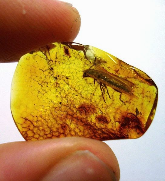
Baltic amber inclusions 50 million years old Length 10 mm.
Amber is heterogeneous in composition, but consists of several resinous bodies more or less soluble in alcohol, ether and chloroform, associated with an insoluble bituminous substance. Amber is a macromolecule by free radical polymerization of several precursors in the labdane family, e.g. communic acid, cummunol, and biformene. These labdanes are diterpenes (C20H32) and trienes, equipping the organic skeleton with three alkene groups for polymerization. As amber matures over the years, more polymerization takes place as well as isomerization reactions, crosslinking and cyclization.
Heated above 200 °C (392 °F), amber suffers decomposition, yielding an “oil of amber”, and leaving a black residue which is known as “amber colophony”, or “amber pitch”; when dissolved in oil of turpentine or in linseed oil this forms “amber varnish” or “amber lac”.
Formation
Molecular polymerization, resulting from high pressures and temperatures produced by overlying sediment, transforms the resin first into copal. Sustained heat and pressure drives off terpenes and results in the formation of amber.
First, the starting resin must be resistant to decay. Many trees produce resin, but in the majority of cases this deposit is broken down by physical and biological process. Exposure to sunlight, rain, and temperate extremes tends to disintegrate resin, and the process is assisted by microorganisms such as bacteria and fungi. For resin to survive long enough to become amber, it must be resistant to such forces or be produced under conditions that exclude them.
Botanical origin
Fossil resins from Europe fall into two categories, the famous Baltic ambers and another that resembles the Agathis group. Fossil resins from the Americas and Africa are closely related to the modern genus Hymenaea, while Baltic ambers are thought to be fossil resins from Sciadopityaceae family plants that used to live in north Europe.
Inclusions
The abnormal development of resin has been called succinosis. Impurities are quite often present, especially when the resin dropped onto the ground, so that the material may be useless except for varnish-making, whence the impure amber is called firniss. Enclosures of pyrites may give a bluish color to amber. The so-called black amber is only a kind of jet. Bony amber owes its cloudy opacity to minute bubbles in the interior of the resin.
In darkly clouded and even opaque amber, inclusions can be imaged using high-energy, high-contrast, high-resolution X-rays.
Classification of Baltic amber by the IAA
Natural Baltic amber – gemstone which has undergone mechanical treatment only (for instance: grinding, cutting, turning or polishing) without any change to its natural properties
Modified Baltic amber – gemstone subjected only to thermal or high-pressure treatment, which changed its physical properties, including the degree of transparency and color, or shaped under similar conditions out of one nugget, previously cut to the required size.
Reconstructed (pressed) Baltic amber – gemstone made of Baltic amber pieces pressed in high temperature and under high pressure without additional components.
Bonded Baltic amber – gemstone consisting of two or more parts of natural, modified or reconstructed Baltic amber bonded together with the use of the smallest possible amount of a colorless binding agent necessary to join the pieces.
Geological record
The oldest amber recovered dates to the Upper Carboniferous period (320 million years ago). Its chemical composition makes it difficult to match the amber to its producers – it is most similar to the resins produced by flowering plants; however, there are no flowering plant fossils until the Cretaceous, and they were not common until the Upper Cretaceous. Amber becomes abundant long after the Carboniferous, in the Early Cretaceous, 150 million years ago, when it is found in association with insects. The oldest amber with arthropod inclusions comes from the Levant, from Lebanon and Jordan. This amber, roughly 125–135 million years old, is considered of high scientific value, providing evidence of some of the oldest sampled ecosystems.
In Lebanon more than 450 outcrops of Lower Cretaceous amber were discovered by Dany Azar a Lebanese paleontologist and entomologist. Among these outcrops 20 have yielded biological inclusions comprising the oldest representatives of several recent families of terrestrial arthropods. Even older, Jurassic amber has been found recently in Lebanon as well. Many remarkable insects and spiders were recently discovered in the amber of Jordan including the oldest zorapterans, clerid beetles, umenocoleid roaches, and achiliid planthoppers.
Baltic amber or succinite (historically documented as Prussian amber) is found as irregular nodules in marine glauconitic sand, known as blue earth, occurring in the Lower Oligocene strata of Sambia in Prussia (in historical sources also referred to as Glaesaria). After 1945 this territory around Königsberg was turned into Kaliningrad Oblast, Russia, where amber is now systematically mined.
It appears, however, to have been partly derived from older Eocene deposits and it occurs also as a derivative phase in later formations, such as glacial drift. Relics of an abundant flora occur as inclusions trapped within the amber while the resin was yet fresh, suggesting relations with the flora of Eastern Asia and the southern part of North America. Heinrich Göppert named the common amber-yielding pine of the Baltic forests Pinites succiniter, but as the wood does not seem to differ from that of the existing genus it has been also called Pinus succinifera. It is improbable, however, that the production of amber was limited to a single species; and indeed a large number of conifers belonging to different genera are represented in the amber-flora.
Paleontological significance
Amber is a unique preservational mode, preserving otherwise unfossilizable parts of organisms; as such it is helpful in the reconstruction of ecosystems as well as organisms; the chemical composition of the resin, however, is of limited utility in reconstructing the phylogenetic affinity of the resin producer.
Amber sometimes contains animals or plant matter that became caught in the resin as it was secreted. Insects, spiders and even their webs, annelids, frogs, crustaceans, bacteria and amoebae, marine microfossils, wood, flowers and fruit, hair, feathers and other small organisms have been recovered in ambers dating to 130 million years ago.
In August 2012, two mites preserved in amber were determined to be the oldest animals ever to have been found in the substance; the mites are 230 million years old and were discovered in north-eastern Italy.
Note : The above story is based on materials provided by Wikipedia 1 & 2.
Google Earth Pro is a 3D interactive globe that can be used to aid planning, analysis and decision making. Businesses, governments and professional users from around the world use Google Earth Pro data visualization, site planning and information sharing tools.
Benefits
Get Productive
With the advanced measuring and drawing tools in Google Earth Pro, you can plan, measure and visualize a site without even leaving your desk.
Make better decisions
Visualize your own information in Google Earth Pro alongside exclusive data layers such as land parcel, demographics and historical traffic data.
Share with others
Create videos in Google Earth Pro that can be shared with stakeholders and customers, providing a unique perspective for any location-based project.
Google Earth Pro key features
Get Productive
With the advanced measuring and drawing tools in Google Earth Pro, you can plan, measure and visualize a site without even leaving your desk.
Distance Measurements
Calculate distance in feet, miles, kilometers, acres, and more. Plan the length of a new runway, the distance between wind turbines, or the circumference of a new commercial retail center.
Area Measurements
Get quick area and radius measurements to determine the buffer zone for an energy plant or the cement needed for a new parking lot.
3D Measurements
Determine the height of a building, measure view sheds from a new residential high-rise to the nearest park, or line-of-sight to the ocean.
Compare Editions
Over the last 10 years, businesses, scientists and hobbyists from all over the world have been using Google Earth Pro for everything from planning hikes to placing solar panels on rooftops. Google Earth Pro has all the easy-to-use features and detailed imagery of Google Earth, along with advanced tools that help you measure 3D buildings, print high-resolution images for presentations or reports, and record HD movies of your virtual flights around the world.
Starting today, even more people will be able to access Google Earth Pro: we’re making it available for free. To see what Earth Pro can do for you—or to just have fun flying around the world—grab a free key and download Earth Pro today. If you’re an existing user, your key will continue to work with no changes required.
This figure shows the number of genes that gained or lost expression in the uterus during the evolution of pregnancy at three major points in mammalian evolution. Credit: Vincent Lynch, Cell Reports
An international team of scientists has identified large-scale genetic changes that marked the evolution of pregnancy in mammals.
They found thousands of genes that evolved to be expressed in the uterus in early mammals, including many that are important for maternal-fetal communication and suppression of the immune system. Surprisingly, these genes appear to have been recruited and repurposed from other tissue types by transposons — ancient mobile genetic elements sometimes thought of as genomic parasites.
The study, published online in Cell Reports on Jan. 29, sheds light on how organisms evolve new morphological structures and functions.
“For the first time, we have a good understanding of how something completely novel evolves in nature, of how this new way of reproducing came to be,” said study author Vincent Lynch, PhD, assistant professor of human genetics at the University of Chicago. “Most remarkably, we found the genetic changes that likely underlie the evolution of pregnancy are linked to domesticated transposable elements that invaded the genome in early mammals. So I guess we owe the evolution of pregnancy to what are effectively genomic parasites.”
To study genetic changes during the evolution of pregnancy in mammals, Lynch and his colleagues used high-throughput sequencing to catalog genes expressed in the uterus of several types of living animals — placental mammals (a human, monkey, mouse, dog, cow, pig, horse and armadillo), a marsupial (opossum), an egg-laying mammal (platypus), a bird, a reptile and a frog. Then they used computational and evolutionary methods to reconstruct which genes were expressed in ancestral mammals.
The researchers found that as the first mammals evolved — and resources for fetal development began to come more from the mother and less from a yolk — hundreds of genes that are important for cellular signaling, metabolism and uterine development started to be expressed in the uterus. As the eggshell was lost and live-birth evolved in the common ancestor to marsupials and placental mammals, more than 1,000 genes were turned on, many of which were strongly linked to the establishment of maternal-fetal communication. As prolonged pregnancy evolved in placental mammals, hundreds of genes began to be expressed that greatly strengthened and elaborated maternal-fetal communication, as well as locally suppressing the maternal immune system in the uterus — thus protecting the developing fetus.
The team also identified hundreds of genes that were turned off as these lineages evolved, many of which had been involved in egg shell formation.
“We found lots of genes important for maintaining hormone signaling and mediating maternal-fetal communication, which are essential for pregnancy, evolved to be expressed in the uterus in early mammals,” Lynch said. “But immune suppression genes stand out. The fetus is genetically distinct from the mother. If these immune genes weren’t expressed in the uterus, the fetus would be recognized by the mother’s immune system as foreign and attacked like any other parasite.”
In addition to function, Lynch and his colleagues investigated the origin of these genes. They found most already had roles in other organ and tissue systems such as the brain, digestive and circulatory systems. But during the evolution of pregnancy, these genes were recruited to be expressed in the uterus for new purposes. They evolved regulatory elements that allowed them to be activated by progesterone, a hormone critical in reproduction.
The team found that this process was driven by ancient transposons — stretches of non-protein coding DNA that can change their position within the genome. Sometimes called “jumping genes,” transposons are generally thought to be genomic parasites that serve only to replicate themselves. Many of the ancient mammalian transposons possessed progesterone binding sites that regulate this process. By randomly inserting themselves into other places in the genome, transposons appear to have passed on this activation mechanism to nearby genes.
“Genes need some way of knowing when and where to be expressed,” Lynch said. “Transposable elements appear to have brought this information, allowing old genes to be expressed in a new location, the uterus, during pregnancy. Mammals very likely have a progesterone-responsive uterus because of these transposons.”
Lynch and his colleagues note their findings represent a novel explanation for how entirely new biological structures and functions arise. Rather than genes gradually evolving uterine expression one at a time, transposable elements coordinated large-scale, genome-wide changes that allowed numerous genes to be activated by the same signal — in this case, progesterone, which helped drive the evolution of pregnancy.
“It’s easy to imagine how evolution can modify an existing thing, but how new things like pregnancy evolve has been much harder to understand,” Lynch said. “We now have a new mechanistic explanation of this process that we’ve never had before.”
Reference:
Vincent J. Lynch, Mauris C. Nnamani, Aurélie Kapusta, Kathryn Brayer, Silvia L. Plaza, Erik C. Mazur, Deena Emera, Shehzad Z. Sheikh, Frank Grützner, Stefan Bauersachs, Alexander Graf, Steven L. Young, Jason D. Lieb, Francesco J. DeMayo, Cédric Feschotte, Günter P. Wagner. Ancient Transposable Elements Transformed the Uterine Regulatory Landscape and Transcriptome during the Evolution of Mammalian Pregnancy. Cell Reports, 2015; DOI: 10.1016/j.celrep.2014.12.052
This global positioning satellite receiver is part of Iceland’s network of 62 such receivers that geoscientists are using to detect movements of the Icelandic crust that are as small as one millimeter per year. Langjökull glacier can be seen in the background. Credit: Richard A. Bennett/ University of Arizona
Earth’s crust under Iceland is rebounding as global warming melts the island’s great ice caps, a University of Arizona-led team reports in an upcoming issue of Geophysical Research Letters.
The paper is the first to show the current fast uplift of the Icelandic crust is a result of accelerated melting of the island’s glaciers and coincides with the onset of warming that began about 30 years ago, the scientists said.
Some sites in south-central Iceland are moving upward as much as 1.4 inches (35 mm) per year — a speed that surprised the researchers.
“Our research makes the connection between recent accelerated uplift and the accelerated melting of the Icelandic ice caps,” said first author Kathleen Compton, a UA geosciences doctoral candidate.
Geologists have long known that as glaciers melt and become lighter, Earth rebounds as the weight of the ice decreases.
Whether the current rebound geologists detect is related to past deglaciation or modern ice loss has been an open question until now, said co-author Richard Bennett, a UA associate professor of geosciences.
“Iceland is the first place we can say accelerated uplift means accelerated ice mass loss,” Bennett said.
To figure out how fast the crust was moving upward, the team used a network of 62 global positioning satellite receivers fastened to rocks throughout Iceland. By tracking the position of the GPS receivers year after year, the scientists “watch” the rocks move and can calculate how far they have traveled — a technique called geodesy.
The new work shows that, at least for Iceland, the land’s current accelerating uplift is directly related to the thinning of glaciers and to global warming.
“What we’re observing is a climatically induced change in Earth’s surface,” Bennett said.
He added there is geological evidence that during the past deglaciation roughly 12,000 years ago, volcanic activity in some regions of Iceland increased thirtyfold.
Others have estimated the Icelandic crust’s rebound from warming-induced ice loss could increase the frequency of volcanic eruptions such as the 2010 eruption of Eyjafjallajökull, which had negative economic consequences worldwide.
The article “Climate driven vertical acceleration of Icelandic crust measured by CGPS geodesy” by Compton, Bennett and their co-author Sigrun Hreinsdóttir of GNS Science in Avalon, New Zealand, was accepted for publication Jan. 14, 2015, and is soon to be published online. The National Science Foundation and the Icelandic Center for Research funded the research.
Some of Iceland’s GPS receivers have been in place since 1995. Bennett, Hreinsdóttir and colleagues had installed 20 GPS receivers in Iceland in 2006 and 2009, thus boosting the coverage of the nation’s geodesy network. In central and southern Iceland, where five of the largest ice caps are located, the receivers are 18 miles (30 km) or less apart on average.
The team primarily used the geodesy network to track geological activity such as earthquakes and volcanic eruptions.
In 2013, Bennett noticed one of long-running stations in the center of the country was showing that site was rebounding at an accelerated rate. He wondered about it, so he and his colleagues checked the nearby stations to see if they had recorded the same changes.
“The striking answer was, yes, they all do,” he said. “We wondered what in the world could be causing this?”
The team began systematically analyzing years of signals from the entire network and found the fastest uplift was the region between several large ice caps. The rate of uplift slowed the farther the receiver was from the ice cap region.
Other researchers had been measuring ice loss and observed a notable uptick in the rate of melting since 1995. Temperature records for Iceland, some of which go back to the 1800s, show temperatures increasing since 1980.
To determine whether the same rate of ice loss year after year could cause such an acceleration in uplift, Compton tested that idea using mathematical models. The answer was no: The glaciers had to be melting faster and faster every year to be causing more and more uplift.
Compton found the onset of rising temperatures and the loss of ice corresponded tightly with her estimates of when uplift began.
“I was surprised how well everything lined up,” she said.
Bennett said, “There’s no way to explain that accelerated uplift unless the glacier is disappearing at an accelerated rate.”
Estimating ice loss is laborious and difficult, he said. “Our hope is we can use current GPS measurements of uplift to more easily quantify ice loss.”
The team’s next step is to analyze the uplift data to reveal the seasonal variation as the ice caps grow during the winter snow season and melt during the summer.
Reference:
Kathleen Compton, Richard A. Bennett, Sigrun Hreinsdóttir. Climate driven vertical acceleration of Icelandic crust measured by CGPS geodesy. Geophysical Research Letters, 2015; DOI: 10.1002/2014GL062446
Note : The above story is based on materials provided by University of Arizona. The original article was written by Mari N. Jensen.