back to top
27.8 C
New York
Sunday, April 20, 2025
Home Blog Page 271

Life can persist in cold, dark world: Life under Antarctic ice explored

The microorganisms that came out of Subglacial Lake Whillans were “incredibly diverse,” and the microbial cells came in a variety of shapes. The yellow arrow points to a rod-shaped cell as seen through a scanning electron microscope. Credit: Image courtesy of WISSARD

The first breakthrough paper to come out of a massive U.S. expedition to one of Earth’s final frontiers shows that there’s life and an active ecosystem one-half mile below the surface of the West Antarctic Ice Sheet, specifically in a lake that hasn’t seen sunlight or felt a breath of wind for millions of years.
The life is in the form of microorganisms that live beneath the enormous Antarctic ice sheet and convert ammonium and methane into the energy required for growth. Many of the microbes are single-celled organisms known as Archaea, said Montana State University professor John Priscu, the chief scientist of the U.S. project called WISSARD that sampled the sub-ice environment. He is also co-author of the MSU author-dominated paper in the Aug. 21 issue of Nature.

“We were able to prove unequivocally to the world that Antarctica is not a dead continent,” Priscu said, adding that data in the Nature paper is the first direct evidence that life is present in the subglacial environment beneath the Antarctic ice sheet.

Lead author Brent Christner said, “It’s the first definitive evidence that there’s not only life, but active ecosystems underneath the Antarctic ice sheet, something that we have been guessing about for decades. With this paper, we pound the table and say, ‘Yes, we were right.'”

Priscu said he wasn’t entirely surprised that the team found life after drilling through half a mile of ice to reach Subglacial Lake Whillans in January 2013. An internationally renowned polar biologist, Priscu researches both the South and North Poles. This fall will be his 30th field season in Antarctica, and he has long predicted the discovery.

More than a decade ago, he published two manuscripts in the journal Science describing for the first time that microbial life can thrive in and under Antarctic ice. Five years ago, he published a manuscript where he predicted that the Antarctic subglacial environment would be the planet’s largest wetland, one not dominated by the red-winged blackbirds and cattails of typical wetland regions in North America, but by microorganisms that mine minerals in rocks at subzero temperatures to obtain the energy that fuels their growth.

Following more than a decade of traveling the world presenting lectures describing what may lie beneath Antarctic ice, Priscu was instrumental in convincing U.S. national funding agencies that this research would transform the way we view the fifth largest continent on the planet.

Although he was not really surprised about the discovery, Priscu said he was excited by some of the details of the Antarctic find, particularly how the microbes function without sunlight at subzero temperatures and the fact that evidence from DNA sequencing revealed that the dominant organisms are archaea. Archaea is one of three domains of life, with the others being Bacteria and Eukaryote.

Many of the subglacial archaea use the energy in the chemical bonds of ammonium to fix carbon dioxide and drive other metabolic processes. Another group of microorganisms uses the energy and carbon in methane to make a living. According to Priscu, the source of the ammonium and methane is most likely from the breakdown of organic matter that was deposited in the area hundreds of thousands of years ago when Antarctica was warmer and the sea inundated West Antarctica. He also noted that, as Antarctica continues to warm, vast amounts of methane, a potent greenhouse gas, will be liberated into the atmosphere enhancing climate warming.

The U.S. team also proved that the microorganisms originated in Lake Whillans and weren’t introduced by contaminated equipment, Priscu said. Skeptics of his previous studies of Antarctic ice have suggested that his group didn’t actually discover microorganisms, but recovered microbes they brought in themselves.

“We went to great extremes to ensure that we did not contaminate one of the most pristine environments on our planet while at the same time ensuring that our samples were of the highest integrity,” Priscu said.

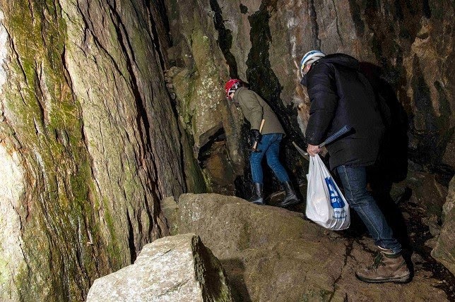
Extensive tests were conducted at MSU two years ago on WISSARD’s borehole decontamination system to ensure that it worked, and Priscu led a publication in an international journal presenting results of these tests. This decontamination system was mated to a one-of-a-kind hot water drill that was used to melt a borehole through the ice sheet, which provided a conduit to the subglacial environment for sampling.

Every day in Antarctica, he would tell his team to keep it simple, Priscu said. To prove that an ecosystem existed below the West Antarctic Ice Sheet, he wanted at least three lines of evidence. They had to see microorganisms under the microscope that came from Lake Whillans and not contaminated equipment. They then had to show that the microorganisms were alive and growing. They had to be identifiable by their DNA.

When the team found those things, he knew they had succeeded, Priscu said.

The Whillans Ice Stream Subglacial Access Research Drilling (WISSARD) project officially began in 2009 with a $10 million grant from the National Science Foundation. Now involving 13 principal investigators at eight U.S. institutions, the researchers drilled down to Subglacial Lake Whillans in January 2013. The microorganisms they discovered are still being analyzed at MSU and other collaborating institutions.

Christner said species are hard to determine in microbiology, but “We are looking at a water column that probably has about 4,000 things we call species. It’s incredibly diverse.”

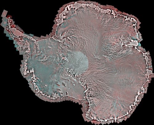
Planning to drill again this austral summer in a new Antarctic location, Priscu said WISSARD was the first large-scale multidisciplinary effort to directly examine the biology of an Antarctic subglacial environment. The Antarctic Ice Sheet covers an area 1 ½ times the size of the United States and contains 70 percent of Earth’s freshwater, and any significant melting can drastically increase sea level. Lake Whillans, one of more than 200 known lakes beneath the Antarctic Ice Sheet and the primary lake in the WISSARD study, fills and drains about every three years. The river that drains Lake Whillans flows under the Ross Ice Shelf, which is the size of France, and feeds the Southern Ocean, where it can provide nutrients for life and influence water circulation patterns.

The opportunity to explore the world under the West Antarctic Ice Sheet is an unparalleled opportunity for the U.S. team, as well as for several MSU-affiliated researchers who are part of that team and wrote or co-authored the Nature paper, Priscu said.

Christner, for one, was a postdoctoral researcher with Priscu and Mark Skidmore at MSU from 2002 through 2006. He is now associate professor of biological sciences at Louisiana State University. Jill Mikucki, now an assistant professor at the University of Tennessee in Knoxville, was one of Priscu’s doctoral students. Skidmore is a glacial geochemist in MSU’s Department of Earth Sciences. Andrew Mitchell, now at Aberystwyth University in the United Kingdom, was a postdoctoral researcher with MSU’s Center for Biofilm Engineering. Alex Michaud and Trista Vick-Majors are currently earning their doctorates in Priscu’s research group at MSU. Other MSU people on the team were Education and Outreach Coordinator Susan Kelly and Project Manager John Sherve.

The fact that MSU was so involved reflects the fact that it is pioneering a new field of science, Priscu said. MSU is the common ancestor of many scientists who study life in and under ice.

“I always tell my students when they come into the lab that ‘We are inventing this field of science. It’s working on life in ice and under ice. This field has never existed before. We thought it up. You are pioneers,'” Priscu said.

Appreciative of the opportunity to participate in WISSARD, Vick-Majors said she saw bacteria under the microscope within an hour after the first sample of water was pulled out of Subglacial Lake Whillans. Within days, she saw proof that the bacteria were active.

“It was very exciting. It will be hard to top,” she said.

She added that, “If you want to do microbial ecology in Antarctic subglacial environments, John is probably the person you want to work with. I feel very lucky to have gotten the opportunity.”

Agreeing, Michaud said, “Some of the graduate students joke, ‘How do we top this?’ We can’t.”

But the students can build on their WISSARD experience and gain a deeper understanding of Subglacial Lake Whillans and other subglacial habitats, he said. It’s not about going out and finding more novel habitats.

Christner said the team that wrote the paper in Nature is the dream team of polar biology. Besides the MSU-affiliated scientists, the co-authors include Amanda Achberger, a graduate student at Louisiana State University; Carlo Barbante, a geochemist at the University of Venice in Italy; Sasha Carter, a postdoctoral researcher at the University of California in San Diego; and Knut Christianson a postdoctoral researcher from St. Olaf College in Minnesota and New York University.

“I hope this exciting discovery will touch the lives (both young and old) of people throughout the world and inspire the next generation of polar scientists,” Priscu said.

Note : The above story is based on materials provided by Montana State University. The original article was written by Evelyn Boswell.

Neither too hot nor too cold: Evolution of marine crocodilians constrained by ocean temperatures

This is a marine crocodilian, here a dyrosaurid, swimming in the warm surface waters during the end of the Cretaceous period. Credit: Guillaume Suan

The ancestors of today’s crocodiles colonised the seas during warm phases and became extinct during cold phases, according to a new Anglo-French study which establishes a link between marine crocodilian diversity and the evolution of sea temperature over a period of more than 140 million years.
The research, led by Dr Jeremy Martin from the Université de Lyon, France and formerly from the University of Bristol, UK is published this week in Nature Communications.

Today, crocodiles are ‘cold-blooded’ animals that mainly live in fresh waters but two notable exceptions, Crocodylus porosus and Crocodylus acutus venture occasionally into the sea. Crocodiles occur in tropical climates, and they are frequently used as markers of warm conditions when they are found as fossils.

While only 23 species of crocodiles exist today, there were hundreds of species in the past. On four occasions in the past 200 million years, major crocodile groups entered the seas, and then became extinct. It is a mystery why they made these moves, and equally why they all eventually went extinct. This new study suggests that crocodiles repeatedly colonized the oceans at times of global warming.

Lead author of the report, Dr Jeremy Martin said: “We thought each of these evolutionary events might have had a different cause. However, there seems to be a common pattern.”

Dr Martin, with a team of paleontologists and geochemists from the Université de Lyon and the University of Bristol, compared the evolution of the number of marine crocodilian fossil species to the sea temperature curve during the past 200 million years. This temperature curve, established using an isotopic thermometer, is widely applied for reconstruction of past environmental conditions and in this case, is based on the isotopic composition of the oxygen contained in the fossilised remains of fossil marine fish (bone, teeth, scales).

Co-author, Christophe Lécuyer explained: “According to this method, it is possible to calculate the temperature of the water in which these fish lived by applying an equation linking the isotopic composition of the fossilised remains to the temperature of mineralisation of their skeleton. The seawater temperatures derived from the composition of fish skeleton thus corresponds to the temperature of water in which the marine crocodiles also lived.”

The results show that colonisation of the marine environment about 180 million years ago was accompanied by a period of global warming of the oceans. These first marine crocodilians became extinct about 25 million years later, during a period of global freezing. Then, another crocodilian lineage appeared and colonised the marine environment during another period of global warming.

The evolution of marine crocodilians is therefore closely tied to the temperature of their medium, and shows that their evolution and their lifestyle, as in modern crocodilians, are constrained by environmental temperatures.

Nevertheless, one fossil lineage does not appear to follow this trend. Jurassic metriorhynchoids did not go extinct during the cold spells of the early Cretaceous, unlike the teleosaurids, another group of marine crocodilians. Quite surprisingly, metriorhynchoids only disappeared a few million years later. This exception will certainly provide grounds for new research, particularly into how the biology of this group adapted to life in the pelagic environment.

Professor Michael Benton from the University of Bristol, another co-author of the study, said: “This work illustrates a case of the impact of climate change on the evolution of animal biodiversity, and shows that for crocodilians, warming phases of our earth’s history constitute ideal opportunities to colonise new environments.”

Note : The above story is based on materials provided by University of Bristol.

Nuclear magnetic resonance experiments using Earth’s magnetic field

Schematic illustration of Earth’s magnetic field. Credit: Courtesy of NASA, Credit/Copyright: Peter Reid, The University of Edinburgh

Earth’s magnetic field, a familiar directional indicator over long distances, is routinely probed in applications ranging from geology to archaeology. Now it has provided the basis for a technique which might, one day, be used to characterize the chemical composition of fluid mixtures in their native environments.
Researchers from the U.S. Department of Energy (DOE)’s Lawrence Berkeley National Laboratory (Berkeley Lab) conducted a proof-of-concept NMR experiment in which a mixture of hydrocarbons and water was analyzed using a high-sensitivity magnetometer and a magnetic field comparable to that of Earth.

The work was conducted in the NMR laboratory of Alexander Pines, one of the world’s foremost NMR authorities, as part of a long-standing collaboration with physicist Dmitry Budker at the University of California, Berkeley, along with colleagues at the National Institute of Standards and Technology (NIST). The work will be featured on the cover of Angewandte Chemie and is published in a paper titled “Ultra-Low-Field NMR Relaxation and Diffusion Measurements Using an Optical Magnetometer.” The corresponding author is Paul Ganssle, who was a PhD student in Pines’ lab at the time of the work.

“This fundamental research program seeks to answer a broad question: how can we sense the interior chemical and physical attributes of an object at a distance, without sampling it or encapsulating it?” says Vikram Bajaj, a principal investigator in Pines’ group. “A particularly beautiful aspect of magnetic resonance is its ability to gently peer within intact objects, but it’s tough to do that from far away.”

High-field and low-field NMR

The exquisite sensitivity of NMR for detecting chemical composition, and the spatial resolution which it can provide in medical applications, requires large and precise superconducting magnets. These magnets are expensive and immobile. Further, the sample of interest must be placed inside the magnet, such that the entire sample is exposed to a homogeneous magnetic field. This well-developed method is called high-field NMR. The sensitivity of high-field NMR is proportional to magnetic field strength.

But chemical characterization of objects that cannot be placed inside a magnet requires a different approach. In ex situ NMR measurements, the geometry of a typical high-field experiment is reversed such that the detector probes the sample surface, and the magnetic field is projected into the object. A main challenge with this situation is generating a homogeneous magnetic field over a sufficiently large sample area: it is not feasible to generate field strengths necessary to make conventional high-resolution NMR measurements.

Instead of a superconducting magnet, low-field NMR measurements may rely on Earth’s magnetic field, given a sufficiently sensitive magnetometer.

“One nice thing about Earth’s magnetic field is that it’s very homogeneous,” explains Ganssle. “The problem with its use in inductively-detected MRI [MRI — magnetic resonance imaging — is NMR’s technological sibling] is that you need a magnetic field that’s both strong and homogeneous, so you need to surround the whole subject with superconducting coils, which is not something that’s possible in an application like oil-well logging.”

“Sensitivity of magnetic resonance depends profoundly on the magnetic field, because the field causes the detected spins to align slightly,” adds Bajaj. “The stronger the applied field, the stronger the signal, and the higher its frequency, which also contributes to the detection sensitivity.”

Paul Ganssle is the corresponding author of a paper in Angewandte Chemie describing ultra-low-field NMR using an optical magnetometer. (Photo by Roy Kaltschmidt)

Earth’s magnetic field is indeed very weak, but optical magnetometers can serve as detectors for ultra-low-field NMR measurements in the ambient field alone without any permanent magnets. This means that ex-situ measurements lose chemical sensitivity due to field strength alone. But this method offers other advantages.

Relaxation and diffusion

In high-field NMR, the chemical properties of a sample are determined from their resonance spectrum, but this is not possible without either extremely high fields or extremely long-lived coherent signals (neither of which are possible with permanent magnets). In contrast, relaxation and diffusion measurements in low-field NMR are more than sufficient to determine bulk materials properties.

“The approach at low-field, which you can achieve using permanent magnets or Earth’s magnetic field, is to measure spin relaxation,” explains Ganssle. Relaxation refers to the rate at which polarized spin returns to equilibrium, based on chemical and physical characteristics of the system. Additionally, NMR experiments resolve chemical compounds based on their different diffusion coefficients, which depend on the size and shape of the molecule.

A key difference between this and conventional experiments is that the relaxation and diffusion properties are resolved through optically-detected NMR, which operates sensitively even in low magnetic fields.

“A previous achievement of our collaboration has been the development of magnetometers for the detection of NMR,” says Bajaj. “This experiment represents the first time magnetometers have been used to make combined relaxation and diffusion measurements of multicomponent mixtures.”

Relaxation and/or diffusion measurements are already commonly used in the oil industry for underground NMR measurements, though conventional probes use a permanent magnet to increase the local magnetic field. There were attempts to perform oil well logging starting in the 1950s using the Earth’s ambient field, but insufficient detection sensitivity led to the introduction of magnets, which are now ubiquitous in logging tools.

“What’s novel here is that using magnetometers, we finally have technology that might be sensitive enough for efficient detection in the Earth’s field, perhaps ultimately enabling detection at longer distances,” explains Scott Seltzer, a co-author on the study.

The design was tested in the lab by measuring relaxation coefficients first for various hydrocarbons and water by themselves, then for a heterogeneous mixture, as well as in two-dimensional correlation experiments, using a magnetometer and an applied magnetic field representative of Earth’s.

“This proof of concept might be productively applied in the oil industry,” says Ganssle. “We mixed hydrocarbons and water, pre-polarized them with a magnet, and applied a magnetic field the same as the Earth’s. Then we made measurements with our magnetometer and determined that we had easily enough sensitivity to separate components of oil and water based on their relaxation spectra.”

This technology could help the oil industry to characterize fluids in rocks, because water relaxes at a different rate from oil. Other applications include measuring the content of water and oil flowing in a pipeline by measuring chemical composition with time, and inspecting the quality of foods and any kind of polymer curing process such as cement curing and drying.

The next step involves understanding the depth in a geological formation that could be imaged with this technology.

“Our next study will be tailored to that question,” says Bajaj. “We hope that this technology will eventually peer a meter or more into the formation and elucidate the chemistry within.”

Eventually, probes could be used to characterize entire borehole environments in this way, while current devices can only image inches deep. The combination of terrestrial magnetism and versatile sensing technology again offers an elegant solution.

Other authors on the Angewandte Chemie paper include Hyun Doug Shin, Micah Ledbetter, Dmitry Budker, Svenja Knappe, John Kitching, and Alexander Pines. The current publication presents some of the work for which Berkeley Lab won an R&D 100 award earlierthis year on optically-detected oil well logging by MRI.

This research was supported by the U.S. Department of Energy’s Office of Science.

Note : The above story is based on materials provided by DOE/Lawrence Berkeley National Laboratory. The original article was written by Rachel Berkowitz.

Thousands of intense earthquakes rock Iceland

This is a Saturday May 8 2010 file image taken from video of a column of ash rising from Iceland’s Eyjafjallajokul volcano. It was reported Tueday Aug. 19, 2014 that thousands of small intense earthquakes are rocking Iceland amid concerns that one of the country’s volcanoes may be close to erupting. Iceland has raised its aviation alert level for the risk of a possible volcanic eruption to orange _ the second-most severe level. The alert is worrisome because of the chaos that followed the April 2010 eruption of Eyjafjallajokul, when more than 100,000 flights were cancelled because volcanic ash floating in the atmosphere is considered an aviation safety hazard. (AP Photo/ APTN)

Thousands of small intense earthquakes are rocking Iceland amid concerns that one of the country’s volcanoes may be close to erupting.

Iceland has raised its aviation alert level for the risk of a possible volcanic eruption to orange—the second-most severe level. The alert is worrisome because of the chaos that followed the April 2010 eruption of Eyjafjallajokul, when more than 100,000 flights were cancelled because volcanic ash floating in the atmosphere is considered an aviation safety hazard.

Some 3,000 earthquakes have taken place since Saturday in Bardarbunga—a subglacial stratovolcano located under Iceland’s largest glacier. Iceland’s Meteorological Office said that no earthquakes above magnitude 3 have been recorded in the last 24 hours.

Seismologists said Tuesday magma is moving, but it is traveling horizontally.

Note : The above story is based on materials provided by © 2014 The Associated Press. All rights reserved.

Has the puzzle of rapid climate change in the last ice age been solved?

Figure A: The Northern Hemisphere in a cold (stadial) phase During the cold stadial periods of the last ice age, massive ice sheets covered northern parts of North America and Europe. Strong northwest winds drove the Arctic sea ice southward, even as far as the French coast. Since the extended ice cover over the North Atlantic prevented the exchange of heat between the atmosphere and the ocean, the strong driving forces for the ocean currents that prevail today were lacking. Ocean circulation, which is a powerful “conveyor belt” in the world’s oceans, was thus much weaker than at present, and consequently transported less heat to northern regions. Map: Alfred-Wegener-Institut Figure A: The Northern Hemisphere in a cold (stadial) phase

Over the past one hundred thousand years cold temperatures largely prevailed over the planet in what is known as the last ice age. However, the cold period was repeatedly interrupted by much warmer climate conditions. Scientists have long attempted to find out why these drastic temperature jumps of up to ten degrees took place in the far northern latitudes within just a few decades.
Now, for the first time, a group of researchers at the Alfred Wegener Institute, Helmholtz Centre for Polar and Marine Research (AWI), have been able to reconstruct these climate changes during the last ice age using a series of model simulations. The surprising finding is that minor variations in the ice sheet size can be sufficient to trigger abrupt climate changes. The new study was published online in the scientific journal Nature last week and will be appearing in the 21 August print issue.

During the last ice age a large part of North America was covered with a massive ice sheet up to 3km thick. The water stored in this ice sheet is part of the reason why the sea level was then about 120 meters lower than today. Young Chinese scientist Xu Zhang, lead author of the study who undertook his PhD at the Alfred Wegener Institute, explains. “The rapid climate changes known in the scientific world as Dansgaard-Oeschger events were limited to a period of time from 110,000 to 23,000 years before present. The abrupt climate changes did not take place at the extreme low sea levels, corresponding to the time of maximum glaciation 20,000 years ago, nor at high sea levels such as those prevailing today – they occurred during periods of intermediate ice volume and intermediate sea levels.” The results presented by the AWI researchers can explain the history of climate changes during glacial periods, comparing simulated model data with that retrieved from ice cores and marine sediments.

During the cold stadial periods of the last ice age, massive ice sheets covered northern parts of North America and Europe. Strong westerly winds drove the Arctic sea ice southward, even as far as the French coast. Since the extended ice cover over the North Atlantic prevented the exchange of heat between the atmosphere and the ocean, the strong driving forces for the ocean currents that prevail today were lacking. Ocean circulation, which is a powerful “conveyor belt” in the world’s oceans, was thus much weaker than at present, and consequently transported less heat to northern regions.

Figure B: The Northern Hemisphere in a warm phase (a brief, warm interstadial phase during glacial climates) During the extended cold phases the ice sheets continued to thicken. When higher ice sheets prevailed over North America, typical in periods of intermediate sea levels, the prevailing northwest winds split into two branches. The major wind field ran to the north of the so-called Laurentide Ice Sheet and ensured that the sea ice boundary off the European coast shifted to the north. Ice-free seas permit heat exchange to take place between the atmosphere and the ocean. At the same time, the southern branch of the northwesterly winds drove warmer water into the ice-free areas of the northeast Atlantic and thus amplified the transportation of heat to the north. The modified conditions stimulated enhanced circulation in the ocean. Consequently, a thicker Laurentide Ice Sheet over North America resulted in increased ocean circulation and therefore greater transportation of heat to the north. The climate in the Northern Hemisphere became dramatically warmer within a few decades until, due to the retreat of the glaciers over North America and the renewed change in wind conditions, it began to cool off again. Map: Alfred-Wegener-Institut

During the extended cold phases the ice sheets continued to thicken. When higher ice sheets prevailed over North America, typical in periods of intermediate sea levels, the prevailing westerly winds split into two branches. The major wind field ran to the north of the so-called Laurentide Ice Sheet and ensured that the sea ice boundary off the European coast shifted to the north. Ice-free seas permit heat exchange to take place between the atmosphere and the ocean. At the same time, the southern branch of the northwesterly winds drove warmer water into the ice-free areas of the northeast Atlantic and thus amplified the transportation of heat to the north. The modified conditions stimulated enhanced circulation in the ocean. Consequently, a thicker Laurentide Ice Sheet over North America resulted in increased ocean circulation and therefore greater transportation of heat to the north. The climate in the Northern Hemisphere became dramatically warmer within a few decades until, due to the retreat of the glaciers over North America and the renewed change in wind conditions, it began to cool off again.

“Using the simulations performed with our climate model, we were able to demonstrate that the climate system can respond to small changes with abrupt climate swings,” explains Professor Gerrit Lohmann, leader of the Paleoclimate Dynamics group at the Alfred Wegener Institute, Germany. In doing so he illustrates the new study’s significance with regards to contemporary climate change. “At medium sea levels, powerful forces, such as the dramatic acceleration of polar ice cap melting, are not necessary to result in abrupt climate shifts and associated drastic temperature changes.”

At present, the extent of Arctic sea ice is far less than during the last glacial period. The Laurentide Ice Sheet, the major driving force for ocean circulation during the glacials, has also disappeared. Climate changes following the pattern of the last ice age are therefore not to be anticipated under today’s conditions.

Figure C: Schematic depiction of current climate conditions in the Northern Hemisphere At present, the extent of the Arctic sea ice is far less than during the last glacial period. The Laurentide Ice Sheet, the major driving force for ocean circulation during the glacials, has also disappeared. Model simulations demonstrate that today’s climate is much more robust in resisting the changes which existed during phases of intermediate ice thickness and intermediate sea levels. It was then, during the last ice age, that the most rapid temperature swings in the Northern Hemisphere took place. Map: Alfred-Wegener-Institut

“There are apparently some situations in which the climate system is more resistant to change while in others the system tends toward strong fluctuations,” summarises Gerrit Lohmann. “In terms of the Earth’s history, we are currently in one of the climate system’s more stable phases. The preconditions, which gave rise to rapid temperature changes during the last ice age do not exist today. But this does not mean that sudden climate changes can be excluded in the future.”

More information:
Xu Zhang, Gerrit Lohmann, Gregor Knorr, Conor Purcell: Abrupt glacial climate shifts controlled by ice sheet changes. Nature, DOI: 10.1038/nature13592

Note : The above story is based on materials provided by Helmholtz Association of German Research Centres

Japan volcanic isle may collapse, create tsunami, study says

Nishino-shima Volcano, Volcano Islands (Japan)

An erupting volcanic island that is expanding off Japan could trigger a tsunami if its freshly-formed lava slopes collapse into the sea, scientists said Tuesday.
The small, but growing, island appeared last year and quickly engulfed the already-existing island of Nishinoshima, around 1,000 kilometres (620 miles) south of Tokyo. It now covers 1.26 square kilometres (0.5 square miles).

The island’s craters are currently spewing out 200,000 cubic metres (7 million cubic feet) of lava every day—enough to fill 80 Olympic swimming pools—which is accumulating in its east, scientists said.

“If lava continues to mount on the eastern area, part of the island’s slopes could collapse and cause a tsunami,” warned Fukashi Maeno, assistant professor of the Earthquake Research Institute at the University of Tokyo.

He said a rockfall of 12 million cubic metres of lava would generate a one metre (three feet) tsunami that could travel faster than a bullet train, hitting the island of Chichijima—130 kilometres away—in around 18 minutes, he said.

Chichijima, home to some 2,000 people, is the largest island in the Ogasawara archipelago, a wild and remote chain that is administratively part of Tokyo.

“The ideal way to monitor and avoid a natural disaster is to set up a new tsunami and earthquake detection system near the island, but it’s impossible for anyone to land on the island in the current situation,” Maeno added.

An official from the Japan Meteorological Agency, which monitors earthquakes and tsunamis, said the agency is watching for any signs of anything untoward.

“We studied the simulation this morning, and we are thinking of consulting with earthquake prediction experts… about the probability of this actually happening, and what kind of measures we would be able to take,” he said.

Japan’s northeast was ravaged by a huge tsunami in March 2011, when a massive undersea earthquake sent a wall of water barrelling into the northeast coast, killing more than 18,000 people and wrecking whole towns.

Note : The above story is based on materials provided by © 2014 AFP

Misunderstood worm-like fossil finds its place in the Tree of Life

Fossil Hallucigenia sparsa from the Burgess Shale Credit: M. R. Smith / Smithsonian Institute

One of the most bizarre-looking fossils ever found — a worm-like creature with legs, spikes and a head difficult to distinguish from its tail — has found its place in the evolutionary Tree of Life, definitively linking it with a group of modern animals for the first time.
The animal, known as Hallucigenia due to its otherworldly appearance, had been considered an ‘evolutionary misfit’ as it was not clear how it related to modern animal groups. Researchers from the University of Cambridge have discovered an important link with modern velvet worms, also known as onychophorans, a relatively small group of worm-like animals that live in tropical forests. The results are published in the advance online edition of the journal Nature.

The affinity of Hallucigenia and other contemporary ‘legged worms’, collectively known as lobopodians, has been very controversial, as a lack of clear characteristics linking them to each other or to modern animals has made it difficult to determine their evolutionary home.

What is more, early interpretations of Hallucigenia, which was first identified in the 1970s, placed it both backwards and upside-down. The spines along the creature’s back were originally thought to be legs, its legs were thought to be tentacles along its back, and its head was mistaken for its tail.

Hallucigenia lived approximately 505 million years ago during the Cambrian Explosion, a period of rapid evolution when most major animal groups first appear in the fossil record. These particular fossils come from the Burgess Shale in Canada’s Rocky Mountains, one of the richest Cambrian fossil deposits in the world.

Looking like something from science fiction, Hallucigenia had a row of rigid spines along its back, and seven or eight pairs of legs ending in claws. The animals were between five and 35 millimetres in length, and lived on the floor of the Cambrian oceans.

A new study of the creature’s claws revealed an organisation very close to those of modern velvet worms, where layers of cuticle (a hard substance similar to fingernails) are stacked one inside the other, like Russian nesting dolls. The same nesting structure can also be seen in the jaws of velvet worms, which are no more than legs modified for chewing.

“It’s often thought that modern animal groups arose fully formed during the Cambrian Explosion,” said Dr Martin Smith of the University’s Department of Earth Sciences, the paper’s lead author. “But evolution is a gradual process: today’s complex anatomies emerged step by step, one feature at a time. By deciphering ‘in-between’ fossils like Hallucigenia, we can determine how different animal groups built up their modern body plans.”

While Hallucigenia had been suspected to be an ancestor of velvet worms, definitive characteristics linking them together had been hard to come by, and their claws had never been studied in detail. Through analysing both the prehistoric and living creatures, the researchers found that claws were the connection joining them together. Cambrian fossils continue to produce new information on origins of complex animals, and the use of high-end imaging techniques and data on living organisms further allows researchers to untangle the enigmatic evolution of earliest creatures.

“An exciting outcome of this study is that it turns our current understanding of the evolutionary tree of arthropods — the group including spiders, insects and crustaceans — upside down,” said Dr Javier Ortega-Hernandez, the paper’s co-author. “Most gene-based studies suggest that arthropods and velvet worms are closely related to each other; however, our results indicate that arthropods are actually closer to water bears, or tardigrades, a group of hardy microscopic animals best known for being able to survive the vacuum of space and sub-zero temperatures — leaving velvet worms as distant cousins.”

“The peculiar claws of Hallucigenia are a smoking gun that solve a long and heated debate in evolutionary biology, and may even help to decipher other problematic Cambrian critters,” said Dr Smith.

Note: The above story is based on materials provided by University of Cambridge. The original story is licensed under a Creative Commons Licence.

Microbes can create dripstones in caves

Tjuv-Ante’s cave seen from the outside looking in. Credit: Image courtesy of University of Southern Denmark

Scientists have found that microscopic organisms can create dripstones in caves. The research illustrates how biological life can influence the formation of Earth’s geology — and the same may be happening right now on other planets.
According to traditional textbooks, dripstones are created by geological or geochemical processes with no influence from living organisms. But now scientists report that formation of dripstones can be a lot more complex than that: Sometimes microbes are responsible for the formation of these geological features.

The researchers from Denmark, Sweden and Spain have investigated dripstone formation in a Swedish cave and conclude that microbes play an active part in their formation.

“If microbes can be responsible for dripstone formation on Earth, the same thing might be happening other places in space,” explains researcher Magnus Ivarsson from Nordic Center for Earth Evolution (NordCEE) at University of Southern Denmark.

The planet Mars is known to be home for a number of caves similar to caves with dripstones created from microbes on Earth. If there are dripstones in these caves, they might have been formed by microbes and thus they are an indication that biological organisms have once lived on Mars.

“If I were a microbe I would definitely live in a cave on Mars,” says Magnus Ivarsson.

He and his colleagues have reported their findings in “International Journal of Speleology.” The colleagues are Therese Sallstedt from NordCEE, University of Southern Denmark, Johannes Lundberg from Swedish Museum of Natural History, Rabbe Sjöberg, retired from Umeå University and Juan Ramon Vidal Romani from University of Coruña in Spain.

The researchers examined dripstones in the Tjuv-Antes cave in Northern Sweden. The cave is 30 meters long and it is home for various kinds of dripstones. When they examined the dripstones the researchers saw distinct layers, mirroring how the dripstones have grown over time and left seasonal layers. Dark layers consist of fossilized microbes and light layers consist of calcite.

The researchers conclude that the microbes were active in the formation of the dripstones.

“Microbes actively contributed to the formation of the dripstones. They didn’t just live on the surface of them,” says Magnus Ivarsson.

Microbes were more active in spring and summer

The layers indicate that the microbes were most active in spring and summer when rain dripped down through the soil and into the cave.

“These drops of water brought nutrients with them, which was consumed by the microbes. As the microbes metabolized they excreted calcium which precipitated and in time helped form the dripstones,” says Magnus Ivarsson.

“Without this microbial activity dripstones would be smaller — or maybe even totally absent,” he adds.

The studying of microbes in caves is not only important for understanding the powers of life on Earth and on other planets. It also has importance for human health:

“Everyday millions of people go into underground caves; metros, train stations, etc. These artificially constructed caves offer some of the same living conditions for microbes as naturally created caves. Health authorities are therefore interested in monitoring and understanding what kind of pathogenic microorganisms can live and grow on the walls of for example metro-stations,” explains Magnus Ivarsson.

Together with Swedish colleagues Magnus Ivarsson is involved in monitoring microbial growth in metro-stations in Stockholm.

Note : The above story is based on materials provided by University of Southern Denmark.

Most complete Antarctic map for climate research made public

Mosaic of satellite images of Antarctica taken by RADARSAT-2. Credit: (RADARSAT-2 Data and Products © MacDonald, Dettwiler and Associates Ltd. (2008) – All Rights Reserved. RADARSAT is an official mark of the Canadian Space Agency.)

The University of Waterloo has unveiled a new satellite image of Antarctica, and the imagery will help scientists all over the world gain new insight into the effects of climate change.
Thanks to a partnership between the Canadian Space Agency (CSA), MacDonald, Dettwiler and Associates Ltd. (MDA), the prime contractor for the RADARSAT-2 program, and the Canadian Cryospheric Information Network (CCIN) at UWaterloo, the mosaic is free and fully accessible to the academic world and the public.

Using Synthetic Aperture Radar with multiple polarization modes aboard the RADARSAT-2 satellite, the CSA collected more than 3,150 images of the continent in the autumn of 2008, comprising a single pole-to-coast map covering all of Antarctica. This is the first such map of the area since RADARSAT-1 created one in 1997.

“The mosaic provides an update on the ever-changing ice cover in this area that will be of great interest to climatologists, geologists, biologists and oceanographers,” said Professor Ellsworth LeDrew, director of the CCIN and a professor in the Faculty of Environment at Waterloo. “When compared to the previous Antarctic RADARSAT-1 mosaic, we can map changes in the icescape with unprecedented accuracy and confidence. Earth’s polar regions are considered a bellwether for the effects of climate change.”

Professor LeDrew is at the forefront of a cultural shift in the way researchers discover, share and preserve their research data. The CCIN links international researchers around the world with numerous government, university and private organizations to provide data and information management infrastructure for the Canadian cryospheric community. This mosaic map of the Antarctic is the latest addition to the CCIN’s Polar Data Catalogue. It is available on the Polar Data Catalogue website. (https://www.polardata.ca/pdcsearch/)

“The Polar Data Catalogue’s mandate is to make such information freely available to scientists, students and the public to enhance our understanding and stewardship of the polar regions,” said Professor LeDrew. “We are proud to work with the Canadian Space Agency and MDA to bring this outstanding Canadian technology and science to the international community.”

Next up for the partnership is a similar mosaic for Greenland, which will provide further crucial information about our shifting climate in the northern hemisphere. There are also plans to continue creating mosaics of Antarctica every few years to provide more data for researchers.

Note : The above story is based on materials provided by University of Waterloo.

Minor variations in ice sheet size can trigger abrupt climate change

New research shows that small fluctuations in the sizes of ice sheets during the last ice age were enough to trigger abrupt climate change. Credit: © Kushnirov Avraham / Fotolia

Small fluctuations in the sizes of ice sheets during the last ice age were enough to trigger abrupt climate change, scientists have found.
The team, which included Cardiff University researchers, compared simulated model data with that retrieved from ice cores and marine sediments in a bid to find out why temperature jumps of up to ten degrees took place in far northern latitudes within just a few decades during the last ice age.

The analysis, led by Germany’s Alfred Wegener Institute Helmholtz Centre for Polar and Marine Research (AWI), is published Aug. 21, 2014 in the scientific journal Nature.

The research confirms that thicker ice sheets increased ocean circulation and transferred more heat to the north due to a redirection of the prevailing winds. As the north warmed, glaciers retreated, the winds returned to normal conditions, and the north became cooler once again, completing the cycle

Conor Purcell from Cardiff University’s School of Earth and Ocean Sciences, said: “Using the simulations performed with our climate model, we were able to demonstrate that the climate system can respond to small changes with abrupt climate swings. Our study suggests that at medium sea levels, powerful forces, such as the dramatic acceleration of polar ice cap melting, are not necessary to create abrupt climate shifts and temperature changes.”

At present, the extent of Arctic sea ice is far less than during the last glacial period. The Laurentide Ice Sheet, the major driving force for ocean circulation during the glacials, has also disappeared. Climate changes following the pattern of the last ice age are therefore not anticipated under today’s conditions.

Professor Gerrit Lohmann, leader of the Paleoclimate Dynamics group at the AWI said: “In terms of the Earth’s history, we are currently in one of the climate system’s more stable phases. The preconditions which gave rise to rapid temperature changes during the last ice age do not exist today, but sudden climate changes cannot be excluded in future.”

Note : The above story is based on materials provided by Cardiff University.

Numbat3D “3D facies models of petroleum reservoirs”

The program encodes a method for generating facies models based on descriptions of outcrops of sedimentary successions or modern analogs of sedimentary systems. The method uses syntactic pattern recognition to encode facies analogs as grammars and a parser to generate stochastic facies models using the information from the grammar.

Channel

The aim of the program is to improve the reconstruction of complexely shaped sand bodies in petroleum reservoirs, particularly those from channelised environments. The facies models are generated as thin 3D layers which can be stacked to form a 3D volume. The parser is a predictive (generative) parser. It is able to condition the facies models to sparse hard data (such as the results of interpretation of poor quality seismic data).

License & Copyright

Copyright © 2009 CSIROThese programs are free software: you can redistribute them and/or modify them under the terms of the GNU General Public License as published by the Free Software Foundation, either version 3 of the License, or (at your option) any later version.

These programs are distributed in the hope that they will be useful, but WITHOUT ANY WARRANTY; without even the implied warranty of MERCHANTABILITY or FITNESS FOR A PARTICULAR PURPOSE. See the GNU General Public License for more details or go to www.gnu.org/licenses

Further Information

Hill, E.J. and Griffiths, C.M., 2009. Describing and generating facies models for reservoir characterisation: 2D map view. Marine and Petroleum Geology. 26, 1554-1563.Hill, E.J., in review. Generating conditioned facies models using a parser with randomised backtracking.

Download:

Numbat3D programs, User Manual and Java source code:
Program: Download
Source Code : Download

Gorges are eradicated by downstream sweep erosion

Credit: Helmholtz Association of German Research Centres

Local surface uplift can block rivers, particularly in mountainous regions. The impounded water, however, always finds its way downstream, often cutting a narrow gorge into the rocks. Subsequent erosion of the rocks can lead to a complete eradication of this initial incision, until not a trace is left of the original breakthrough. In extreme cases the whole gorge disappears, leaving behind a broad valley with a flat floodplain. Previously, the assumption was that this transition from a narrow gorge to a wide valley was driven by gorge widening and the erosion of the walls of the gorges.

A team of scientists from the GFZ German Research Centre for Geosciences in Potsdam has now revealed a new mechanism that drives this process of fluvial erosion. The geoscientists analyzed the development of a gorge on the Da’an Chi river in Taiwan over a period of almost ten years. There, uplift that was caused by the Jiji earthquake of 1999 (magnitude 7.6), and that runs transverse to the river, had formed a blockage. Earthquakes of that size occur there every 300 to 500 years. “Before the quake there was no sign of a gorge at all in this riverbed, which is one and a half kilometers wide”, explains Kristen Cook of the GFZ. “We have here the world’s first real-time observation of the evolution of gorge width by fluvial erosion over the course of several years.” Currently the gorge is roughly a kilometer long, 25 meters wide and up to 17 meters deep. Initially, the gorge walls were eroded at a rate of five meters per year, and today are still retreating one and a half meters per year.

The scientists identified a hitherto unknown mechanism by which the gorge is destroyed. “Downstream sweep erosion” they termed this process. “A wide braided channel upstream of the gorge is necessary,” explains co-author Jens Turowski (GFZ). “The course of this channel changes regularly and it has to flow in sharp bends to run into the gorge. In these bends, the bed-load material that is transported by the river hits the upper edge of the gorge causing rapid erosion.” This mechanism gradually washes away all of the bedrock surrounding the gorge and, therefore, is the cause for the planation of the riverbed over the complete width of the valley. Assuming the current erosion rate of 17 meters per year, it will take here at the Da’an Chi River only 50 to 100 years until again a flat beveled channel again fills the valley. In contrast, lateral erosion in the gorge would be too slow to eradicate the gorge in the time of one earthquake cycle. The newly discovered downstream sweep erosion is far more effective.

More information:
Kristen L. Cook, Jens M. Turowski and Niels Hovius: “River gorge eradication by downstream sweep erosion”, Nature Geoscience, Advance Online Publication, 17.08.2014, DOI: 10.1038/ngeo2224

Note : The above story is based on materials provided by Helmholtz Association of German Research Centres

Syr Darya

Astronaut photograph of the Syr Darya River floodplain

Table of Contents

The Syr Darya is a river in Central Asia. The second part of the name (Darya) means river, though “Syr Darya River” is the conventional name. The current name dates only from the 18th century; since roughly the Muslim Conquests of Central Asia the river was known as the Seyhun (سيحون) River, i.e., one of the four rivers of Jannah, or paradise. Prior to the coming of Islam to Central Asia, the river’s name is recorded by several sources, including those relating to Alexander the Great as the Jaxartes River.

Name

The earliest recorded name comes down to us as Jaxartes /ˌdʒæɡˈzɑrtiːz/ or Iaxartes /ˌaɪ.əɡˈzɑrtiːz/ (Ἰαξάρτης) in Ancient Greek. The Greek preserves the Old Persian name Yakhsha Arta (“True Pearl”), perhaps a reference to the color of its glacially-fed water. More evidence for the Persian etymology comes from its Turkic name up to the time of the Arab Conquest, the Yinchu, or Pearl, River.

Following the Conquests, the river appears in the sources uniformly as the Seyhun (سيحون), one of the four rivers flowing from Jannah.

The Turkic and current name of the River, Syr (Sïr), does not appear before the 16th century. In the 17th century, Abu al-Ghazi Bahadur Khan, historian and ruler of Khiva, calls the Aral Sea the “Sea of Sïr,” or Sïr Tengizi.

Geography

Map of the watershed of Syr Darya. Aral Sea boundaries are c. 1960.

The river rises in two headstreams in the Tian Shan Mountains in Kyrgyzstan and eastern Uzbekistan—the Naryn River and the Kara Darya which come together in the Uzbek part of the Fergana Valley—and flows for some 2,212 kilometres (1,374 mi) west and north-west through Uzbekistan and southern Kazakhstan to the remains of the Aral Sea. The Syr Darya drains an area of over 800,000 square kilometres (310,000 sq mi), but no more than 200,000 square kilometres (77,000 sq mi) actually contribute significant flow to the river. Its annual flow is a very modest  37 cubic kilometres (30,000,000 acre·ft) per year—half that of its sister river, the Amu Darya.

Along its course, the Syr Darya irrigates the most productive cotton-growing region in the whole of Central Asia, together with the towns of Kokand, Khujand, Kyzylorda and Turkestan.

Various local governments throughout history have built and maintained an extensive system of canals. These canals are of central importance in this arid region. Many fell into disuse in the 17th and early 18th cnetury, but the Khanate of Kokand rebuilt many in the 19th century, primarily along the Upper and Middle Syr Darya.

Massive expansion of irrigation canals in Middle and Lower Syr Darya during the Soviet period to water cotton and rice fields caused ecological damage to the area. The amount of water taken from the river was such that in some periods of the year, no water at all reaches the Aral Sea, similar to the Amu Darya situation in Uzbekistan and Turkmenistan.

Note : The above story is based on materials provided by Wikipedia

Earth’s early life endured long asteroid bombardment

The dinosaurs had it easy (Image: Detlev Van Ravenswaay/SPL)

IT WAS a blitzkrieg with no let-up. Earth may have been pounded by massive asteroids for a billion years longer than we thought, with the impacts only stopping about 3 billion years ago. If that is true, early life had to endure a bombardment that periodically melted Earth’s surface.
The planet formed 4.5 billion years ago, and chunks of rock many kilometres across continued falling onto it for hundreds of millions of years. It seemed there was a final burst of impacts around 3.9 billion years ago – and by 3.8 billion years ago it was all over. The first fossils of life are very slightly younger.

That story is wrong, says Donald Lowe of Stanford University in California. The barrage continued far longer. “Its termination was not an abrupt drop-off but a gradual waning until 3 billion years ago,” he says.

Lowe and his colleagues have spent 40 years studying a patch of ancient rocks in eastern South Africa called the Barberton Belt. Over 25 years ago they found four layers of spherical particles, which seemed to have condensed from clouds of vaporised rock. Lowe says they are the traces of four major meteorite impacts, and date from between 3.5 and 3.2 billion years ago.

Now Lowe’s team have described another four layers of spherules from the same period. That means there were eight major impacts within about 250 million years, bolstering the case that the bombardment was still going on (Geology, doi.org/t48).

The moon also bears scars of major impacts up to 3 billion years ago, says William Bottke of the Southwest Research Institute in Boulder, Colorado. “This makes it unavoidable that the Earth was still getting hit by big things late in the game,” he says.

The impacts were on a scale beyond anything that Earth has experienced since the dawn of complex animals. The asteroid believed to have finished off the dinosaurs left a layer of spherules a few millimetres thick. “Our layers are 30 to 40 centimetres,” says Lowe. That suggests the asteroids were at least 20 kilometres across and possibly more than 70. “They were big boys,” says Lowe.

Each impact would have flung huge amounts of rock and gas into the air and blasted a crater 400 to 800 kilometres across. Lowe recently calculated that one such impact would have caused an earthquake that went on for many minutes and tsunamis that could have circled the entire planet.

Such impacts would wipe out most animals and plants if they happened today, but back then all life was single-celled. “We don’t know if this was apocalyptic for the microbes,” says Lowe. Those on the far side of the planet “would have to ride out some large waves” and a rain of hot rocks, but some would surely have survived.

One major group of microbes would have been at more risk: photosynthetic bacteria, which had to live near the surface of the ocean where there was plenty of light. “A very large impact has the potential to evaporate the top 100 metres of the ocean,” says Lowe. “The atmosphere would have heated up to hundreds of degrees Celsius. That would be apocalyptic. If you evaporate below the photic zone, you would obliterate photosynthesis.”

It’s a definite possibility, says Bottke. Such severe impacts could help explain why the air became rich in oxygen only around 2.4 billion years ago. Oxygen is a waste product of photosynthesis, and photosynthetic bacteria may not have been able to gain a foothold on the early Earth under such heavy bombardment. Bottke says there may have been a “back and forth battle”, with life “fighting sporadic setbacks” from asteroid impacts.

Note : The above story is based on materials provided by Michael Marshall “newscientist”

Fossilized marine plankton tell the tale of the end Permian mass extinction

Artist’s impression of the Siberian Traps at the time of the Permian mass extinction. Credit: José-Luis Olivares/MIT

The worst mass extinction the Earth has ever seen occurred 252 million years ago. The boundary of the Permian and Triassic geological periods marked the demise of around 90 percent of marine species and 70 percent of land species.
Solving the intricate puzzles of mass extinctions is vital when it comes to understanding the external factors that could hinder life on other planets. Several theories have been proposed to explain this mass extinction, but scientists believe that the most likely trigger for this mass extinction was one of the largest volcanic eruptions ever recorded.

A paper by Qinglai Feng and Thomas Algeo entitled “Evolution of oceanic redox conditions during the Permo-Triassic transition: Evidence from deepwater radiolarian facies,” recently accepted in the journal Earth-Science Reviews details how tiny marine plankton known as radiolarians are shedding light on the sequence of events that led to this mass extinction.

In this scenario, a mantle plume rose from deep within the Earth and burst through the crust at Siberia. It didn’t just form one volcano, rather it was an event known as a flood basalt eruption. Lava poured from fissures over an area the size of Europe and this period of volcanic activity lasted between one and two million years. Today this area is known as the Siberian Traps.

Depletion of oxygen in the oceans

The gases and ash that spewed out caused catastrophic changes to the environment by initiating a greenhouse effect. The extra carbon dioxide, methane and water vapor in the atmosphere retained more radiation from the Sun, and global temperatures rose by between 10 to 15 degrees Celsius (18 to 27 degrees Fahrenheit). This increase in temperature ultimately caused the oxygen levels in the oceans to become dangerously low, a condition known as anoxia. There are several factors that contributed to the widespread ocean anoxia that exterminated so many species during the transition from the Permian to the Triassic.

The rising temperatures were a major factor as oxygen becomes less soluble in water as temperatures increase. The increased heat also warmed the surface waters more than usual. As warmer water is lower in density than cold water, the density difference between the deep layers and the surface increased. This hindered the layers of water from mixing, and thus contributed to the depletion in oxygen.

In the atmosphere, the volcanic gases mixed with water to form acid rain, which decimated forests and left the soil with no roots to keep it in place. Intensified weathering then washed this soil, along with extra nutrients, into the ocean. The additional nutrients in the water encouraged the growth of algae, which increased the amount of organic matter that sank into the ocean depths. The decay process of this organic matter consumed oxygen, and depleted the oxygen faster than it could be replenished.

Radiolarians

Understanding the sequence of events that took place in a mass extinction hundreds of millions of years ago is no easy task. One way to learn how oxygen levels impacted ancient life is to study the fossils of marine plankton known as radiolarians.

Radiolarians are marine plankton that are widespread throughout the oceans and have persisted from the Cambrian period (540 million years ago) to modern times. The distribution of these single-celled floating organisms is controlled by the conditions in the ocean, such as temperature, depth, and the amount of oxygen.

The skeletons of radiolarians are well preserved, even in deep water sediments. Different orders of radiolarians thrive at different depths in the ocean, so they make a good study subject in investigations on how extinctions were related to the depth of the water.

The level of oxygen in the prehistoric oceans can be measured from the mineralogy of the rocks in which the fossils are found. When the radiolarians were abundant during the Permian, the rocks were red in color due to the presence of hematite. Hematite is an iron oxide and an indicator that oxygen was plentiful in the ocean at this time. Later in the Permian, the rocks become gray or black in color. The hematite was replaced with pyrite, which is a mineral deposited in an anoxic environment.

Multiple mass extinctions

The varying diversity of radiolarians found in fossils shows that the mass extinction occurred in several stages. The rocks also showed that anoxic events likely occurred after major ash fall events. Multiple anoxic events were recorded in rocks in different regions around the globe throughout the late Permian and early Triassic. Each event coincided with enhanced extinction rates that resulted in sudden drops in the level of diversity, creating a “stepwise” mass extinction.

Fossils discovered in southern China reveal that the number of shallow water species of radiolarians increased from 85 to 125, known as a species radiation event. The cause of this radiation event is uncertain, but may be due to an increase in the diversity of suitable environments for the radiolarians to thrive.

Soon after this irradiation of species, the first extinction occurred. This was a precursor to the main mass extinction that wiped out most marine species. The number of species of radiolarians found in the Chinese rocks dwindled from 125 to 15. This precursor extinction annihilated species, rather than entire genera, although some of the remaining genera only had one surviving species.

“One characteristic of such volcanic systems is that they tend to have a short ‘lead-in’ time of activity prior to the main eruption, followed by a period of pulsed eruptive activity one to two million years following the main eruption,” says Thomas Algeo. “This pattern seems to fit observations for the Permian-Triassic crisis, and there is increasing evidence of intensification of marine environmental stresses prior to the main extinction event.”

When the main eruption occurred, more species were lost, but this time the extinction rates were also large at the genus level. Anoxia spread through the Panthalassa Ocean that once surrounded the supercontinent of Pangea, as well as the Paleo-Tethys ocean, which was nestled within the C-shaped Pangea. Oxygen was severely depleted at low and intermediate depths, particularly at low latitudes.

Shallow waters were only briefly subjected to anoxic conditions and some shallow waters, particularly those at mid to high latitudes, would have been a refuge for marine life. Evidence for this lies in the fact that radiolarians had a greater survival rate at higher latitudes.

Dead clade walking

After the main extinction at the end of the Permian, the number of radiolarians had been dramatically depleted on a global scale. The widespread anoxia that marked the end of the Permian persisted for a short time after the main extinction, and further anoxic events occurred intermittently for the next two million years. These additional anoxic events meant that the mass extinctions were not yet over for the radiolarians, and more genera disappeared during the early Triassic .Groups that had survived the main mass extinction were then annihilated, a phenomenon known as “dead clade walking.”

Later in the Triassic, oxic conditions returned to the oceans and the radiolarians and other marine species recovered. New groups of radiolarians evolved, and they spread out to reclaim both shallow and deep waters of the oceans.

Note : The above story is based on materials provided by Astrobio.net
This story is republished courtesy of NASA’s Astrobiology Magazine. Explore the Earth and beyond at www.astrobio.net .

São Francisco River

The São Francisco (Portuguese pronunciation: [sɐ̃w fɾɐ̃ˈsiʃku]) is a river in Brazil. With a length of 2,914 kilometres (1,811 mi), it is the longest river that runs entirely in Brazilian territory, and the fourth longest in South America and overall in Brazil (after the Amazon, the Paraná and the Madeira). It used to be known as the Opara by the indigenous people before colonisation, and is today also known as Velho Chico (“Old Frank”).

São Francisco river basin

The São Francisco originates in the Canastra mountain range in the central-western part of the state of Minas Gerais. It runs generally north in the states of Minas Gerais and Bahia, behind the coastal range, draining an area of over 630,000 square kilometres (240,000 sq mi), before turning east to form the border between Bahia on the right bank and the states of Pernambuco and Alagoas on the left one. After that, it forms the boundary between the states of Alagoas and Sergipe and washes into the Atlantic Ocean. In addition to the five states which the São Francisco directly traverses or borders, its drainage basin also includes tributaries from the state of Goiás and the Federal District.

It is an important river for Brazil, called “the river of national integration” because it unites diverse climes and regions of the country, in particular the Southeast with the Northeast. It is navigable between the cities of Pirapora (Minas Gerais) and Juazeiro (Bahia), as well as between Piranhas (Alagoas) and the mouth on the ocean, but traditional passenger navigation has all but disappeared in recent years due to changes in the river flow.

Discovery

The river was first discovered by Europeans on 4 October 1501 (by the Florentine discoverer Amerigo Vespucci, who named it after Saint Francis of Assisi, whose feast day falls on 4 October).

In 1865 the British explorer and diplomat Richard Francis Burton was transferred to Santos in Brazil. He explored the central highlands, canoeing down the São Francisco river from its source to the falls of Paulo Afonso.

The four parts of the São Francisco River

The course of the river, running through five states, may be divided into four parts, as follows:

  1. The high part, from its source to Pirapora in Minas Gerais
  2. The upper middle part, from Pirapora, where the navigable part begins, up to Remanso (Bahia) and the Sobradinho Dam
  3. The lower middle part, from the Sobradinho dam to Paulo Afonso, also in Bahia (bordering on Alagoas), and ending at the Itaparica Dam
  4. The low part, from Paulo Afonso to the river’s mouth on the Atlantic Ocean

Tributaries

The river obtains water from 168 rivers and streams, of which 90 are on the right bank and 78 on the left bank. The main tributaries are:

  • Paraopeba River
  • Abaeté River
  • Das Velhas River
  • Jequitaí River
  • Paracatu River
  • Urucuia River
  • Verde Grande River
  • Carinhanha River
  • Corrente River
  • Grande River

Note : The above story is based on materials provided by Wikipedia

Study of Chilean quake shows potential for future earthquake

The Iquique earthquake took place on the northern portion of the subduction zone formed when the Nazca tectonic plate slides under the South American plate. Credit: USGS

Near real-time analysis of the April 1 earthquake in Iquique, Chile, showed that the 8.2 event occurred in a gap on the fault unruptured since 1877 and that the April event was not what the scientists had expected, according to an international team of geologists.
“We assumed that the area of the 1877 earthquake would eventually rupture, but all indications are that this 8.2 event was not the 8.8 event we were looking for,” said Kevin P. Furlong, professor of geophysics, Penn State. “We looked at it to see if this was the big one.”

But according to the researchers, it was not. Seismologists expect that areas of faults will react the same way over and over. However, the April earthquake was about nine times less energetic than the one in 1877 and was incapable of releasing all the stress on the fault, leaving open the possibility of another earthquake.

The Iquique earthquake took place on the northern portion of the subduction zone formed when the Nazca tectonic plate slides under the South American plate. This is one of the longest uninterrupted plate boundaries on the planet and the site of many earthquakes and volcanos. The 8.2 earthquake was foreshadowed by a systematic sequence of foreshocks recorded at 6.0, 6.5, 6.7 and 6.2 with each foreshock triggering the next until the main earthquake occurred.

These earthquakes relieved the stresses on some parts of the fault. Then the 8.2 earthquake relieved more stress, followed by a series of aftershocks in the range of 7.7. While the aftershocks did fill in some of the gaps left by the 8.2 earthquake, the large earthquake and aftershocks could not fill in the entire gap where the fault had not ruptured in a very long time. That area is unruptured and still under stress.

The foreshocks eased some of the built up stress on 60 to 100 miles of fault, and the main shock released stress on about 155 miles, but about 155 miles of fault remain unchanged, the researchers report today (Aug. 13) in Nature.

“There can still be a big earthquake there,” said Furlong. “It didn’t release the total hazard, but it told us something about this large earthquake area. That an 8.8 rupture doesn’t always happen.”

The researchers were able to do this analysis in near real time because of the availability of large computing power and previously laid groundwork.

The computing power allowed researchers to model the fault more accurately. In the past, subduction zones were modeled as if they were on a plane, but the plate that is subducting curves underneath the other plate creating a 3-dimensional fault line. The researchers used a model that accounted for this curving and so more accurately recreated the stresses on the real geology at the fault.

“One of the things the U.S. Geological Survey and we have been doing is characterizing the major tectonic settings,” said Furlong. “So when an earthquake is imminent, we don’t need a lot of time for the background.”

In essence, they are creating a library of information about earthquake faults and have completed the first level, a general set of information on areas such as Japan, South America and the Caribbean. Now they are creating the levels of north and south Japan or Chile, Peru and Ecuador.

Knowing where the old earthquake occurred, how large it was and how long ago it happened, the researchers could look at the foreshocks, see how much stress they relieved and anticipate, at least in a small way, what would happen.

“This is what we need to do in the future in near real time for decision makers,” said Furlong.

Note : The above story is based on materials provided by Penn State. The original article was written by A’ndrea Elyse Messer.

South-west diversity still a mystery but comparison lends clues

WA’s south-west has higher species richness but fewer genera than the south-east of Australia. Credit: Arthur Chapman

A WA botanist says detailed fossil records and the development of phylogenetic trees could help experts understand why flora in Australia’s south-west is so diverse in comparison to the south-east.
Curator of WA Herbarium at the Department of Parks and Wildlife Kevin Thiele has confirmed in research that WA’s south-west has higher species richness but fewer genera than the south-east of Australia.

Dr Thiele says experts cannot yet explain the reasons for the special characteristics of the flora in the south-west, but more critical thinking and research will help to discriminate between possible explanations.

The collaborative research reviewed explanations behind south-west diversity, with one possibility being “supercharged speciation” that occurred in the south-west and not the south-east.

Alternatively, Dr Thiele says unlike the south-east, Australia’s south-west could have been environmentally stable for a long period of time.

“Even though the rate at which new species are generated in the south-west and south-east may be approximately equal, it may be that fewer species have gone extinct in the south-west over a long period of time,” he says.

However, Dr Thiele says the special nature of the flora in the south-west might not be historical and could be due to the soil of each area.

“The very richest parts of the south-west are areas that are on very nutrient-poor oligotrophic soils,” he says.

“These soils are a real challenge to grow on and it’s a common observation in many parts of the world that these types of very nutrient limited of sandy soils seem to have quite rich floras on them.”

Dr Thiele says developing phylogenies for flora in the two areas may help because particularly with molecular phylogenies, they can be dated to some extent.

“We might be able to see things like a difference in the phylogenetic patterns in the south-west and south-east,” he says.

Dr Thiele says there is not a good understanding of fossil history in the south-west of Australia however work done in south-east Australia has used fossil records of an old flora from before the ice ages.

He says the records show the flora was just as rich as the flora in south-western Australia, but much of it went extinct.

“That is beginning to suggest that perhaps there has been a greater extinction in the south-east,” he says.

However, Dr Thiele says even if there was great extinction during the ice ages, it doesn’t explain why the south-east is richer in genera.

More information: 
Dr Thiele describes the findings in a paper published in the Journal of the Royal Society of Western Australia, June 2014.

Note : The above story is based on materials provided by Science Network WA

Indus River

Satellite image of the Indus River basin in Pakistan, India, and China.

The Indus River is a major river in Asia which flows through Pakistan. It also has courses through western Tibet and Northern India. Originating in the Tibetan Plateau in the vicinity of Lake Mansarovar, the river runs a course through the Ladakh region of Jammu and Kashmir, towards Gilgit and Baltistan and then flows in a southerly direction along the entire length of Pakistan to merge into the Arabian Sea near the port city of Karachi in Sindh. The total length of the river is 3,180 km (1,980 mi). It is Pakistan’s longest river.
The river has a total drainage area exceeding 1,165,000 km2 (450,000 sq mi). Its estimated annual flow stands at around 207 km3 (50 cu mi), making it the twenty-first largest river in the world in terms of annual flow. The Zanskar is its left bank tributary in Ladakh. In the plains, its left bank tributary is the Chenab which itself has four major tributaries, namely, the Jhelum, the Ravi, the Beas and the Sutlej. Its principal right bank tributaries are the Shyok, the Gilgit, the Kabul, the Gomal and the Kurram. Beginning in a mountain spring from Nepal and fed with glaciers and rivers in the Himalayas, the river supports ecosystems of temperate forests, plains and arid countryside.

The Indus forms the delta of present-day Pakistan mentioned in the Vedic Rigveda as Sapta Sindhu and the Iranian Zend Avesta as Hapta Hindu (both terms meaning “seven rivers”). The river has been a source of wonder since the Classical Period, with King Darius of Persia sending Scylax of Caryanda to explore the river as early as 510 BC.

Description

The Indus River provides key water resources for the economy of Pakistan – especially the Breadbasket of Punjab province, which accounts for most of the nation’s agricultural production, and Sindh. The word Punjab means “land of five rivers” and the five rivers are Jhelum, Chenab, Ravi, Beas and Sutlej, all of which finally merge in Indus. The Indus also supports many heavy industries and provides the main supply of potable water in Pakistan.

The ultimate source of the Indus is in Tibet; it begins at the confluence of the Sengge and Gar rivers that drain the Nganglong Kangri and Gangdise Shan mountain ranges. The Indus then flows northwest through Ladakh and Baltistan into Gilgit, just south of the Karakoram range. The Shyok, Shigar and Gilgit rivers carry glacial waters into the main river. It gradually bends to the south, coming out of the hills between Peshawar and Rawalpindi. The Indus passes gigantic gorges 4,500–5,200 metres (15,000–17,000 feet) deep near the Nanga Parbat massif. It flows swiftly across Hazara and is dammed at the Tarbela Reservoir. The Kabul River joins it near Attock. The remainder of its route to the sea is in the plains of the Punjab and Sindh, where the flow of the river becomes slow and highly braided. It is joined by the Panjnad at Mithankot. Beyond this confluence, the river, at one time, was named the Satnad River (sat = “seven”, nadī = “river”), as the river was now carrying the waters of the Kabul River, the Indus River and the five Punjab rivers. Passing by Jamshoro, it ends in a large delta to the east of Thatta.

The Indus is one of the few rivers in the world to exhibit a tidal bore. The Indus system is largely fed by the snows and glaciers of the Himalayas, Karakoram and the Hindu Kush ranges of Tibet, the Indian state of Jammu and Kashmir and the Northern Areas of Pakistan respectively. The flow of the river is also determined by the seasons – it diminishes greatly in the winter, while flooding its banks in the monsoon months from July to September. There is also evidence of a steady shift in the course of the river since prehistoric times – it deviated westwards from flowing into the Rann of Kutch and adjoining Banni grasslands after the 1816 earthquake.

The traditional source of the river is the Senge Khabab or “Lion’s Mouth”, a perennial spring, not far from the sacred Mount Kailash, and is marked by a long low line of Tibetan chortens. There are several other tributaries nearby which may possibly form a longer stream than Senge Khabab, but unlike the Senger Khabab, are all dependent on snowmelt. The Zanskar River which flows into the Indus in Ladakh has a greater volume of water than the Indus itself before that point.

“That night in the tent [next to Senge Khabab] I ask Sonmatering which of the Indus tributaries which we crossed this morning is the longest. All of them, he says, start at least a day’s walk away from here. The Bukhar begins near the village of Yagra. The Lamolasay’s source is in a holy place: there is a monastery there. The Dorjungla is a very difficult and long walk, three days perhaps, and there are many sharp rocks; but it its water is clear and blue, hence the tributary’s other name, Zom-chu, which Karma Lama translates as ‘Blue Water’. The Rakmajang rises from a dark lake called the Black Sea.
One of the longest tributaries — and thus a candidate for the river’s technical source — is the Kla-chu, the river we crossed yesterday by bridge. Also known as the Lungdep Chu, it flows into the Indus from the south-east, and rises a day’s walk from Darchen. But Sonamtering insists that the Dorjungla is the longest of the ‘three types of water’ that fall into the Seng Tsanplo [‘Lion River’ or Indus].”

Geography

Tributaries

  • Nagar River
  • Astor River
  • Balram River
  • Dras River
  • Gar River
  • Ghizar River
  • Gilgit River
  • Gomal River
  • Kabul River
  • Kurram River
  • Panjnad River
  • Shigar River
  • Shyok River
  • Soan River
  • Tanubal River
  • Zanskar River
  • Jhelum River
  • Ravi River
  • Chenab River
  • Beas River
  • Satluj River

Geology

The Indus river feeds the Indus submarine fan, which is the second largest sediment body on the Earth at around 5 million cubic kilometres of material eroded from the mountains. Studies of the sediment in the modern river indicate that the Karakoram Mountains in northern Pakistan and India are the single most important source of material, with the Himalayas providing the next largest contribution, mostly via the large rivers of the Punjab (Jhelum, Ravi, Chenab, Beas and Sutlej). Analysis of sediments from the Arabian Sea has demonstrated that prior to five million years ago the Indus was not connected to these Punjab rivers which instead flowed east into the Ganges and were captured after that time. Earlier work showed that sand and silt from western Tibet was reaching the Arabian Sea by 45 million years ago, implying the existence of an ancient Indus River by that time. The delta of this proto-Indus river has subsequently been found in the Katawaz Basin, on the Afghan-Pakistan border.

In the Nanga Parbat region, the massive amounts of erosion due to the Indus river following the capture and rerouting through that area is thought to bring middle and lower crustal rocks to the surface.

Note : The above story is based on materials provided by Wikipedia

Midwestern Fault Zones Are Still Alive

Earthquakes occurring today in the New Madrid Seismic Zone (center of image; red dots denote quakes greater than magnitude 3 that have occurred since 1974) are not aftershocks of massive quakes that occurred in the winter of 1811 to 12, a new study suggests. Credit : U.S. Geological Survey

The occasional quakes rattling the New Madrid Seismic Zone, a series of midwestern faults named for a small town in the Missouri Bootheel, aren’t aftershocks of the massive quakes that rocked our fledgling nation more than 2 centuries ago, a new study suggests. The analysis reinvigorates a debate about the true level of seismic risk that those fault zones pose.
In the winter of 1811 to 1812, a series of colossal quakes—by some estimates among the strongest ever seen in what is today the continental United States—exploded beneath what is now the American Midwest. In a span of less than 2 months, four magnitude-7 or greater temblors struck along a zigzag set of faults centered near the river town of New Madrid, Missouri, the closest settlement to the destruction. Although the quakes were felt as far away as the East Coast, the area around the quake was sparsely populated, so devastation was limited. (The Greater St. Louis area, home to about 2.9 million people today but less than 6000 at the time the quakes occurred, is centered about 235 kilometers north of New Madrid.)

As with all major quakes, the New Madrid quakes spawned a lot of aftershocks, says Morgan Page, a geophysicist with the U.S. Geological Survey (USGS) in Pasadena, California. Indeed, one of the four largest quakes of that winter—one that occurred at about dawn on 16 December 1811—is considered to be an aftershock of the first quake in the series, which occurred about 5 hours earlier. One of seismology’s biggest debates, which bears on the amount of seismic risk in the area today, is how long those aftershocks continued. Some studies suggest that they’re still going on, which would support those who argue there is little chance of major quakes striking New Madrid in coming centuries.

A new analysis by Page and USGS colleague Susan Hough indicates that modern-day rumblings in the New Madrid Seismic Zone are not echoes of the 1811 to 1812 quakes, however. Instead, they are signs the seismic zone is still alive and kicking. The team’s analysis uses a model that simulates how series of aftershocks unfold—statistics that were first described by a Japanese seismologist in the 1890s. (According to that model, the number and size of aftershocks generally decrease over time in a predictable way.)

For the new study, Page and Hough considered three sets of data: the number and size of the original set of quakes, the number and spacing of magnitude-6 or larger aftershocks recorded in the years after the original group of temblors, and the number and size of magnitude-4 or larger quakes recorded by seismometers in the region today. Results of the team’s statistical analysis suggest that the long-verified, more-than-a-century-old model doesn’t fit the pattern of seismicity seen on the New Madrid Seismic Zone in the past 2 centuries, the researchers report online today in Science.

Specifically, the team found that if today’s magnitude-4 or larger quakes were truly aftershocks of the 1811 to 1812 quakes, then scientists should have seen about 135 magnitude-6 or larger temblors between 1812 and 2012. In fact, Page says, only two such quakes occurred. Conversely, a series of aftershocks that contains only two such moderate-sized aftershocks would also contain far fewer magnitude-4 or larger quakes than sensors actually record today. In other words, modern-day quakes are signs that the faults in the region are still accumulating stress—and sometimes releasing it as fresh rumblings.

But some scientists don’t find the team’s results convincing. For example, aftershock sequences for quakes that occur at faults far from a tectonic plate boundary—such as the New Madrid Seismic Zone—often last much longer than those triggered by quakes near plate boundaries, says Seth Stein, a geophysicist at Northwestern University in Evanston, Illinois. Because those faults behave differently, he contends, the new study doesn’t show that modern-day quakes aren’t aftershocks.

Stein and Mian Liu, a geophysicist at the University of Missouri, Columbia, find that GPS equipment installed throughout the region has failed to detect strain building up in Earth’s crust that would be required to trigger fresh quakes. That would suggest that the New Madrid threat is not growing, but the source of seismic stress in the region, far from any boundaries where tectonic plates jostle and scrape past each other, isn’t clear. Some scientists have argued that Earth’s crust in northern portions of North America is still slowly springing upward in response to the melting of the ice sheet that smothered the region during the last ice age. As that rebound slows, so should the buildup of stress in the crust underlying the Midwest, they say. For this reason, Stein and other scientists have in the past suggested that the New Madrid Seismic Zone is gradually dying.

But previous studies don’t show seismicity in the region to be slowing down, at least over the very long term. Indeed, groups of major quakes strike the New Madrid Seismic Zone with some regularity, Page says. Geologic evidence shows that other clusters of large quakes rumbled the region around 900 A.D. and around 1450, she notes. But that recent seismic history doesn’t help predict when the next set of “big ones” will occur, or how large they’ll be. “These things don’t go off on a regular basis,” she adds.

Based on previous analyses, USGS scientists have estimated the chance of having an earthquake similar to one of the 1811 to 1812 temblors in the next 50 years is about 7% to 10%, and the chance of having a magnitude-6 or larger earthquake in the next 50 years is 25% to 40%.

Note : The above story is based on materials provided by Sid Perkins ” American Association for the Advancement of Science “

Related Articles