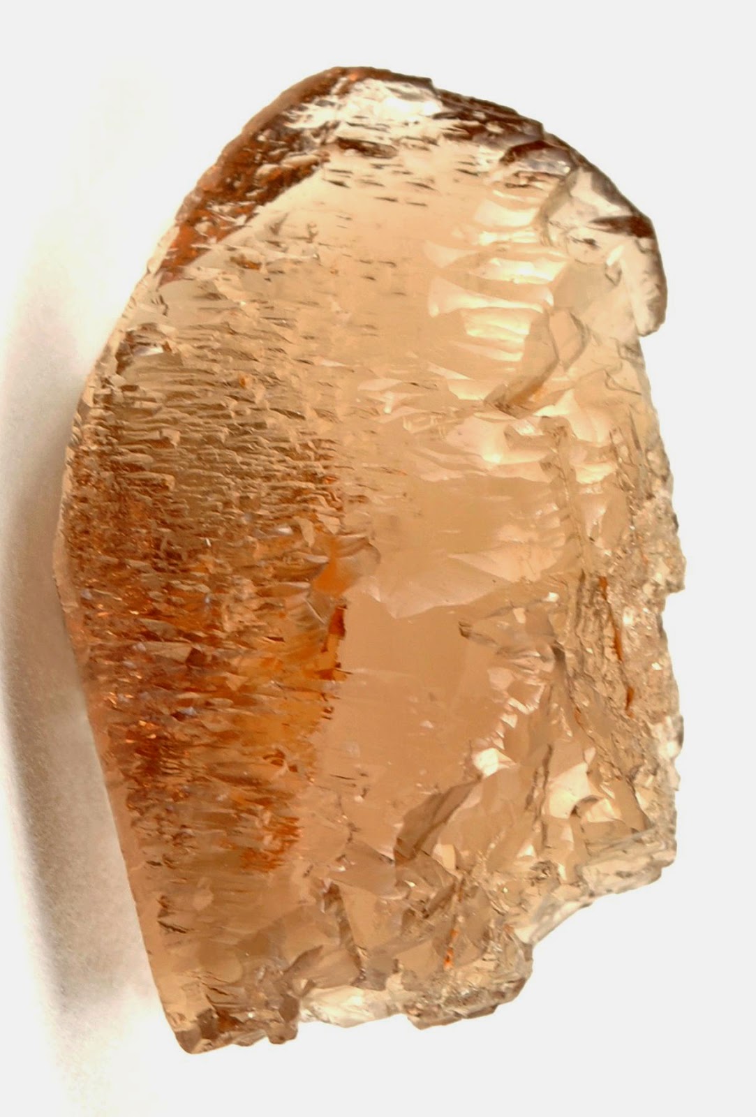
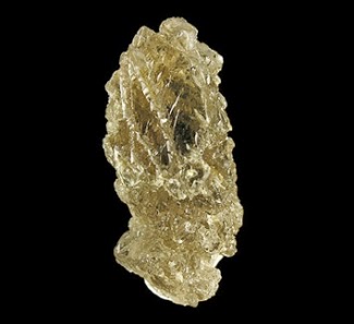
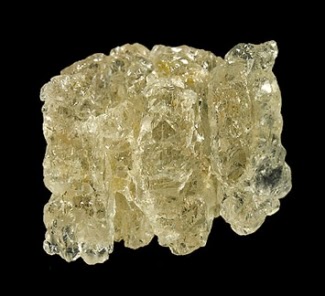
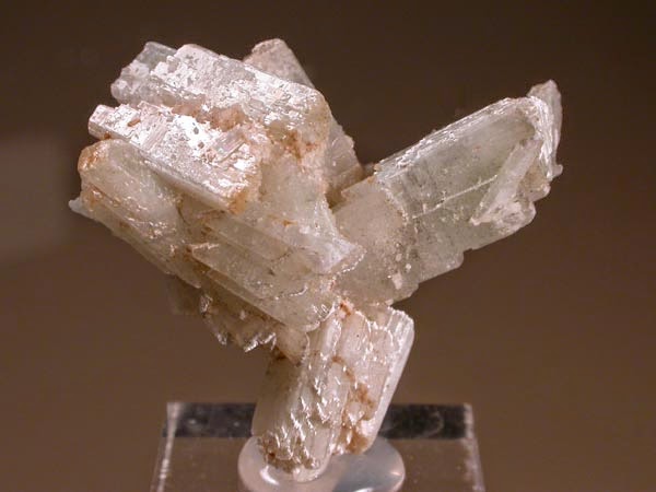
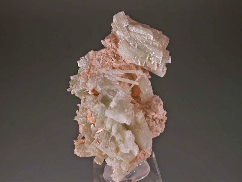
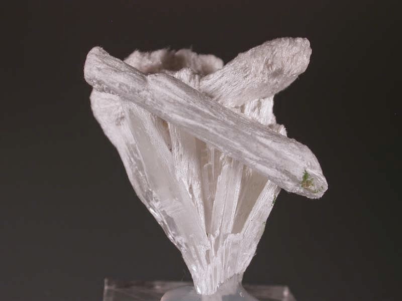
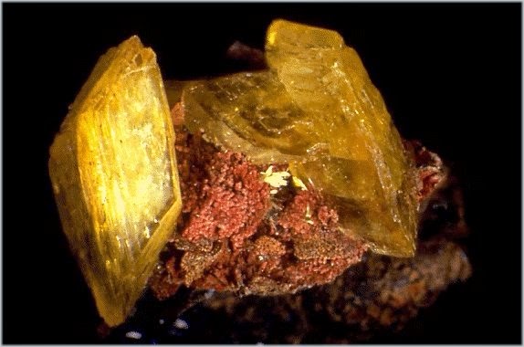
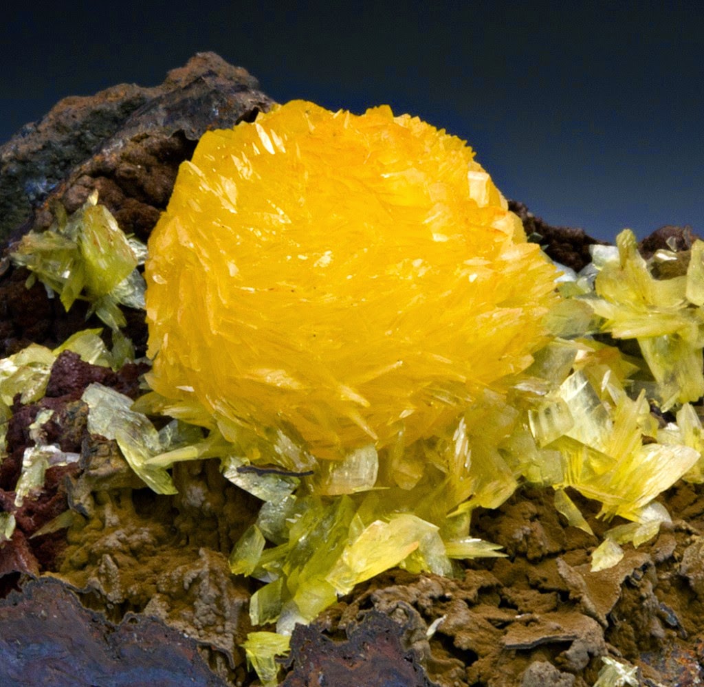
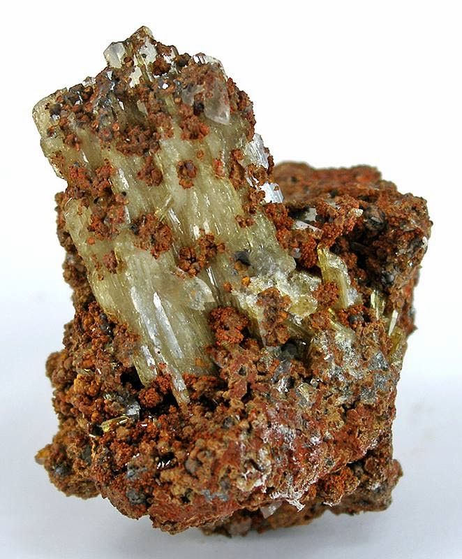
Chemical Formula: LiAl(Si4O10) Name Origin: From the Greek petalon – “leaf” in allusion to the perfect basal cleavage.
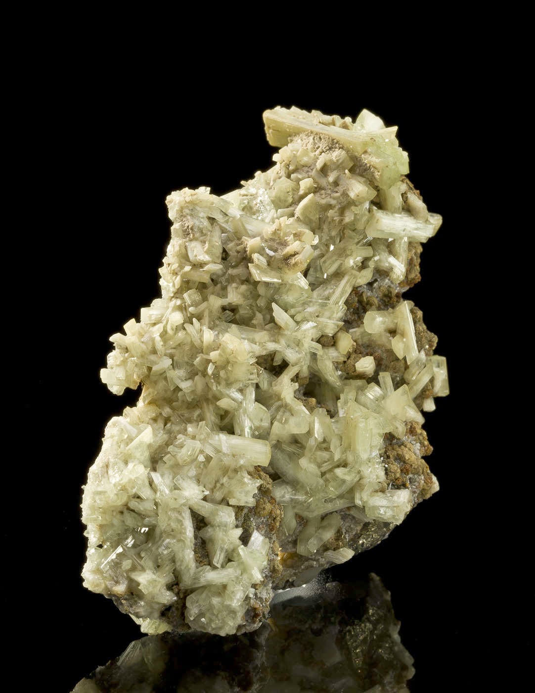
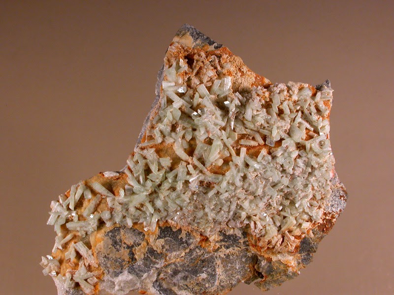
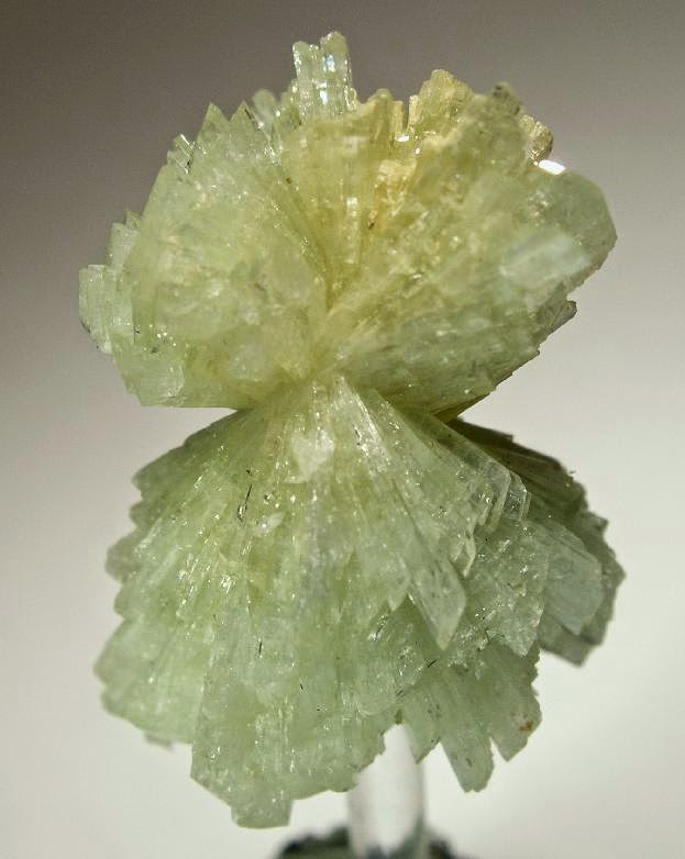
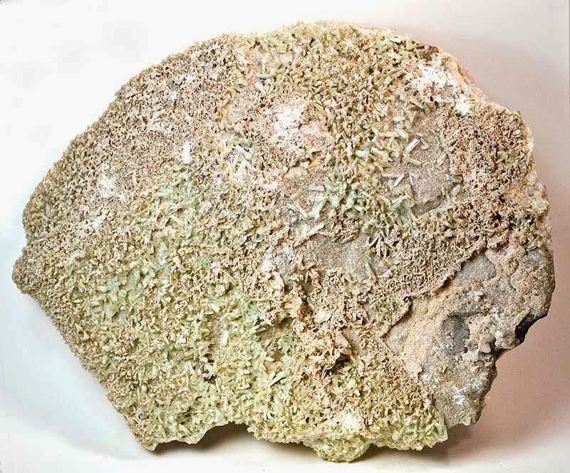
Petalite, also known as castorite, is a lithium aluminium phyllosilicate mineral LiAl(Si4O10), crystallizing in the monoclinic system. Petalite is a member of the feldspathoid group. It occurs as colourless, grey, yellow, yellow grey, to white tabular crystals and columnar masses. Occurs in lithium-bearing pegmatites with spodumene, lepidolite, and tourmaline.
Petalite is an important ore of lithium, and is converted to spodumene and quartz by heating to ~500 °C and under 3 kbar of pressure in the presence of a dense hydrous alkali borosilicate fluid with a minor carbonate component. The colorless varieties are often used as gemstones.
Discovery and occurrence
Discovered in 1800, type locality: Utö Island, Haninge, Stockholm, Sweden. The name is derived from the Greek word petalon, which means leaf.
Economic deposits of petalite ahre found near Kalgoorlie, Western Australia; Aracuai, Minas Gerais, Brazil; Karibib, Namibia; Manitoba, Canada; and Bikita, Zimbabwe.
The first important economic application for petalite was as a raw material for the glass-ceramic cooking ware CorningWare. It has been used as a raw material for ceramic glazes.
History
Discovery date : 1800 Town of Origin : ILE UTO Country of Origin : SUEDE
Optical properties
Refractive Index: from 1,50 to 1,52 Axial angle 2V: 82-84°
Physical properties
Hardness: 6,50 Density : from 2,41 to 2,42 Color : colorless; white; grey; yellowish grey; yellow; reddish; greenish; pink Luster: vitreous; nacreous Streak : white Break: sub-conchoidal Cleavage : Yes
Salamanders served as hosts: This reconstruction shows how scientists think the fly larvae adhered to the skin of the amphibian. Credit: Yang Dinghua, Nanjing
Researchers from the University of Bonn and from China have discovered a fossil fly larva with a spectacular sucking apparatus.
Around 165 million years ago, a spectacular parasite was at home in the freshwater lakes of present-day Inner Mongolia (China): A fly larva with a thorax formed entirely like a sucking plate. With it, the animal could adhere to salamanders and suck their blood with its mouthparts formed like a sting. To date no insect is known that is equipped with a similar specialised design. The international scientific team is now presenting its findings in the journal eLIFE.
The parasite, an elongate fly larva around two centimeters long, had undergone extreme changes over the course of evolution: The head is tiny in comparison to the body, tube-shaped with piercer-like mouthparts at the front. The mid-body (thorax) has been completely transformed underneath into a gigantic sucking plate; the hind-body (abdomen) has caterpillar-like legs. The international research team believes that this unusual animal is a parasite which lived in a landscape with volcanoes and lakes what is now northeastern China around 165 million years ago. In this fresh water habitat, the parasite crawled onto passing salamanders, attached itself with its sucking plate, and penetrated the thin skin of the amphibians in order to suck blood from them.
“The parasite lived the life of Reilly,” says Prof. Jes Rust from the Steinmann Institute for Geology, Mineralogy and Palaeontology of the University of Bonn. This is because there were many salamanders in the lakes, as fossil finds at the same location near Ningcheng in Inner Mongolia (China) have shown. “There scientists had also found around 300,000 diverse and exceptionally preserved fossil insects,” reports the Chinese scientist Dr. Bo Wang, who is researching in palaeontology at the University of Bonn as a PostDoc with sponsorship provided by the Alexander von Humboldt Foundation. The spectacular fly larva, which has received the scientific name of “Qiyia jurassica,” however, was a quite unexpected find. “Qiyia” in Chinese means “bizarre”; “jurassica” refers to the Jurassic period to which the fossils belong.
A fine-grained mudstone ensured the good state of preservation of the fossil
For the international team of scientists from the University of Bonn, the Linyi University (China), the Nanjing Institute of Geology and Palaeontology (China), the University of Kansas (USA) and the Natural History Museum in London (England), the insect larva is a spectacular find: “No insect exists today with a comparable body shape,” says Dr Bo Wang. That the bizarre larva from the Jurassic has remained so well-preserved to the present day is partly due to the fine-grained mudstone in which the animals were embedded. “The finer the sediment, the better the details are reproduced in the fossils,” explains Dr Torsten Wappler of the Steinmann-Institut of the University of Bonn. The conditions in the groundwater also prevented decomposition by bacteria.
Astonishingly, no fossil fish are found in the freshwater lakes of this Jurassic epoch in China. “On the other hand, there are almost unlimited finds of fossilised salamanders, which were found by the thousand,” says Dr Bo Wang. This unusual ecology could explain why the bizarre parasites survived in the lakes: fish are predators of fly larvae and usually hold them in check. “The extreme adaptations in the design of Qiyia jurassica show the extent to which organisms can specialise in the course of evolution,” says Prof. Rust.
As unpleasant as the parasites were for the salamanders, their deaths were not caused by the fly larvae. “A parasite only sometimes kills its host when it has achieved its goal, for example, reproduction or feeding ,” Dr Wappler explains. If Qiyia jurassica had passed through the larval stage, it would have grown into an adult insect after completing metamorphosis. The scientists don’t yet have enough information to speculate as to what the adult it would have looked like, and how it might have lived.
Note : The above story is based on materials provided by Universität Bonn.
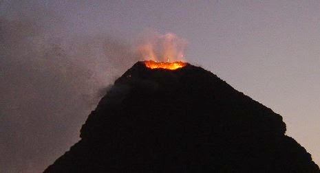
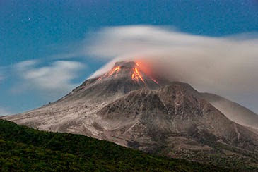
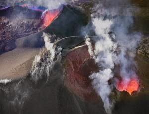
Guatemala’s Pacaya volcano needs monitoring to prevent death and destruction from eruptions and landslides, and Michigan Technological University researchers are helping local residents and government agencies do just that.
As part of a two-year, $100,000 project, Thomas Oommen, Gregory Waite, and Rüdiger Escobar-Wolf have joined their Guatemalan counterparts scouting the countryside around the volcano to come up with the best sites for monitoring equipment. It’s the first step in compiling information to set up equipment for volcanic monitoring, part of a Society of Exploration Geophysicists-Geoscientists Without Borders (SEG-GWB) project.
“The infrastructure is not there,” said Oommen, assistant professor of geological and mining engineering and sciences. “They lack proper instrumentation, and we will overcome this challenge with seismic stations, GPS, high-resolution cameras and other devices to capture the data.”
They’ll also produce permanent displays explaining volcanic hazards and monitoring to inform local people and visiting tourists.
Oommen just returned from Guatemala, where he, geophysicist Waite and geological engineering postdoc Escobar-Wolf met with leadership of that country’s National Institute of Seismology, Volcanology, Meteorology, and Hydrology (INSIVUMEH), which monitors atmospheric, geophysical and hydrological phenomena and makes recommendations in case of natural disasters.
Monitoring Pacaya Volcano
The team also met with a group from the Instituto Geografico Nacional (IGN), which has ongoing studies of ground deformation around Pacaya, to discuss how best to integrate the new instrumentation with their existing monitoring program.
“The idea is to train the local agencies in the use of the equipment, so we can turn it over to them some day,” Oommen said. “The data obtained from this equipment will help several PhD students here to advance research on volcanic hazards.”
In addition to the work with these scientific agencies, a key meeting was held with leaders of the Pacaya National Park, the municipality of the area that surrounds the volcano, and the representatives from National Coordination Agency for Disaster reduction (CONRED), an agency responsible for risk reduction from a variety of hazards.
“These groups were all very keen to cooperate on the monitoring and outreach components of the project,” said Waite. “The success of this project hinges on this collaboration.”
The project also includes funding for thesis projects to be developed by students from San Carlos University in Guatemala, using the data that will be produced by the new monitoring equipment.
“The multidisciplinary approach involving the volcanologists at INSIVUMEH, the administration of the National Park, the academics from the San Carlos University, and collaborators in other agencies has a great potential to further that type of cooperation beyond the scope of this two-year project,” said Escobar-Wolf.
Pacaya is one of the most active volcanoes in Central America, Oommen pointed out.
“It erupted recently, so the project is timely,” he said. “They’ve had to evacuate 9,000 people 11 times in 24 years. These are large events.”
He said that real-time streaming of data can help prevent a catastrophic event, especially with better monitoring of data. It’s part of volcanic research that goes back some fifty years.
“[Professor Emeritus] Bill Rose actually started this work in Guatemala in the 1960s,” Oommen said. “This is a continuation of natural hazard reduction with a humanitarian focus.”
“I got my undergraduate degree at the San Carlos University and worked for CONRED before coming to Michigan Tech” said Escobar-Wolf. “I also worked with INSIVUMEH at Pacaya and other volcanoes, and I first came in contact with Tech researchers and students, led by Bill Rose. It is very rewarding to collaborate in this project with some of the same people I studied and worked with when I was in Guatemala.”
This research-come-full-circle is a three-pronged attack, Oommen said: build the capacities of local emergency agencies, improve understanding of volcanic hazards at Pacaya, and validate and advance the remote-sensing-based research, including graduate student research back on the Michigan Tech campus.
Note : The above story is based on materials provided by Michigan Technological University
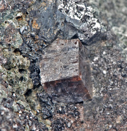
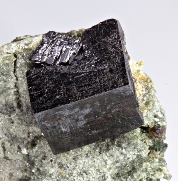
Chemical Formula: CaTiO3 Locality: Achmatovsk near Kussinsk in the Zlatoust district, Ural mountans, Russia. Name Origin: Named after the Russian mineralogist, L. A. Perovski (1792-1856).
Perovskite (pronunciation: pe’ɹovskaɪt) is a calcium titanium oxide mineral species composed of calcium titanate, with the chemical formula CaTiO3. The mineral was discovered in the Ural Mountains of Russia by Gustav Rose in 1839 and is named after Russian mineralogist Lev Perovski (1792–1856).
It lends its name to the class of compounds which have the same type of crystal structure as CaTiO3 known as the perovskite structure. The perovskite crystal structure was first described by Victor Goldschmidt in 1926, in his work on tolerance factors. The crystal structure was later published in 1945 from X-ray diffraction data on barium titanate by the Irish crystallographer Helen Dick Megaw.
Occurrence
Perovskite is found in contact carbonate skarns at Magnet Cove, Arkansas. It occurs in altered blocks of limestone ejected from Mount Vesuvius. It occurs in chlorite and talc schist in the Urals and Switzerland. It is also found as an accessory mineral in alkaline and mafic igneous rocks, nepheline syenite, melilitite, kimberlites and rare carbonatites. Perovskite is a common mineral in the Ca-Al-rich inclusions found in some chondritic meteorites.
A rare earth-bearing variety, knopite, (Ca,Ce,Na)(Ti,Fe)O3) is found in alkali intrusive rocks in the Kola Peninsula and near Alnö, Sweden. A niobium-bearing variety, dysanalyte, occurs in carbonatite near Schelingen, Kaiserstuhl, Germany.
History
Discovery date : 1839 Town of Origin : ACHMATOVSK, DISTRICT DE SLATOUST, MTS OURAL Country of Origin : RUSSIE ex-URSS
Optical properties
Optical and misc. Properties: Fragile, cassant – Transparent – Opaque – Translucide Refractive Index : 2,34
Physical properties
Hardness: 5,50 Density: 4,01 Color : black; brown; yellow; brown red; grayish black; amber; yellow brown Luster: adamantine; metallic; greasy; unpolished Streak : white; grey Break: sub-conchoidal; irregular Cleavage: Yes
The Soufrière Hills volcano, Montserrat Credit: Dr Henry Odbert
A new special volume documenting volcanology research developed at Montserrat, West Indies and including major contributions from University of Bristol researchers is published this month by the Geological Society of London.
The Eruption of the Soufrière Hills Volcano, Montserrat from 2000 to 2010, edited by G. Wadge, R.E.A. Robertson and B. Voight, comprises 27 substantial chapters that review the development and application of scientific study at the Soufrière Hills Volcano. It follows from an earlier memoir, published in 2002, and represents the most complete collection and description of this extraordinary eruption and the breadth of scientific investigation it has facilitated.
In the mid-1990s, the small island of Montserrat in the Caribbean made international news when the Soufrière Hills Volcano began erupting after about 400 years of inactivity. The ensuing eruption has caused devastation on the island – almost all of the population were displaced and the capital city, Plymouth, has subsequently been destroyed and partly buried by volcanic ash. Unlike many eruptions of its type, the Soufrière Hills eruption has been long-lived, continuing to erupt on and off since 1995.
When the volcano first showed signs of unrest, scientists from all over the world scrambled to make measurements and observations. There has been particularly strong involvement from UK scientists, owing to Montserrat’s status as a UK Overseas Territory. With its unique setting and unusual longevity, the Montserrat eruption has become one of the most important and best-studied eruptions of its type, and has spurned a substantive contribution to volcanological science.
Scientists at the University of Bristol have been central to research on Montserrat, on topics ranging from the physics and chemistry of volcanism to developing monitoring and analysis techniques.
In particular, Professor Willy Aspinall and Professor Steve Sparks pioneered the application of operational quantitative risk assessment for volcanic hazards at Montserrat. The models, which are still used in Montserrat, represent the longest-running and most sophisticated volcanic risk assessment of their kind.
Dr Henry Odbert, a research associate in the School of Earth Sciences and former scientist at the Montserrat Volcano Observatory, has authored several chapters in the memoir, including a review and analysis of cyclic eruptive behaviour – one of the notable characteristics of the Montserrat eruption.
His chapter on geodetic observation on Montserrat, with contributions from Dr Jo Gottsmann and Dr Stefanie Hautmann, presents a comprehensive review of how geophysical study enables us to better understand the deep physical processes of volcanic eruptions. Dr Hautmann leads a chapter describing investigation of the volcanic system using gravity data.
The eruption on Montserrat has enabled scientific study that has yielded substantive contributions to our understanding of how volcanic eruptions work, how we can best monitor and interpret volcanic behaviour, and how to assess and manage the risks posed by volcanic hazards.
Dr Odbert said: “This collection, with significant contribution from researchers at the University of Bristol, presents an overview of the science associated with the eruption on Montserrat, particularly between 2000 and 2010 – the last time the volcano erupted fresh lava. At the time of writing, the volcano continues to indicate that future eruptions are still possible. A major scientific challenge now is to apply our knowledge and understanding of this fascinating volcano to forecast how the eruption may evolve hereafter.”
Note : The above story is based on materials provided by University of Bristol
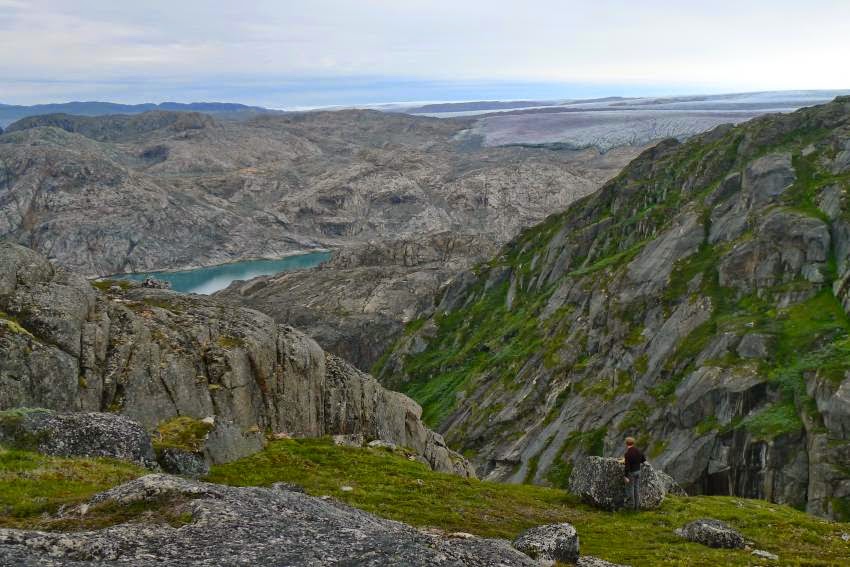
Co-author Anders Carlson (Oregon State University) conducting field research at the south Greenland ice sheet at its inland margin near Narsaq. The new study by Reyes and colleagues suggests that much of southern Greenland was nearly ice-free during a long period of warmer-than-present climate about 400,000 years ago. Credit: Alberto Reyes
A new study suggests that a warming period more than 400,000 years ago pushed the Greenland ice sheet past its stability threshold, resulting in a nearly complete deglaciation of southern Greenland and raising global sea levels some 4-6 meters.
The study is one of the first to zero in on how the vast Greenland ice sheet responded to warmer temperatures during that period, which were caused by changes in the Earth’s orbit around the sun.
Results of the study, which was funded by the National Science Foundation, are being published this week in the journal Nature.
“The climate 400,000 years ago was not that much different than what we see today, or at least what is predicted for the end of the century,” said Anders Carlson, an associate professor at Oregon State University and co-author on the study. “The forcing was different, but what is important is that the region crossed the threshold allowing the southern portion of the ice sheet to all but disappear.
“This may give us a better sense of what may happen in the future as temperatures continue rising,” Carlson added.
Few reliable models and little proxy data exist to document the extent of the Greenland ice sheet loss during a period known as the Marine Isotope Stage 11. This was an exceptionally long warm period between ice ages that resulted in a global sea level rise of about 6-13 meters above present. However, scientists have been unsure of how much sea level rise could be attributed to Greenland, and how much may have resulted from the melting of Antarctic ice sheets or other causes.
To find the answer, the researchers examined sediment cores collected off the coast of Greenland from what is called the Eirik Drift. During several years of research, they sampled the chemistry of the glacial stream sediment on the island and discovered that different parts of Greenland have unique chemical features. During the presence of ice sheets, the sediments are scraped off and carried into the water where they are deposited in the Eirik Drift.
“Each terrain has a distinct fingerprint,” Carlson noted. “They also have different tectonic histories and so changes between the terrains allow us to predict how old the sediments are, as well as where they came from. The sediments are only deposited when there is significant ice to erode the terrain. The absence of terrestrial deposits in the sediment suggests the absence of ice.
“Not only can we estimate how much ice there was,” he added, “but the isotopic signature can tell us where ice was present, or from where it was missing.”
This first “ice sheet tracer” utilizes strontium, lead and neodymium isotopes to track the terrestrial chemistry.
The researchers’ analysis of the scope of the ice loss suggests that deglaciation in southern Greenland 400,000 years ago would have accounted for at least four meters – and possibly up to six meters – of global sea level rise. Other studies have shown, however, that sea levels during that period were at least six meters above present, and may have been as much as 13 meters higher.
Carlson said the ice sheet loss likely went beyond the southern edges of Greenland, though not all the way to the center, which has not been ice-free for at least one million years.
In their Nature article, the researchers contrasted the events of Marine Isotope Stage 11 with another warming period that occurred about 125,000 years ago and resulted in a sea level rise of 5-10 meters. Their analysis of the sediment record suggests that not as much of the Greenland ice sheet was lost – in fact, only enough to contribute to a sea level rise of less than 2.5 meters.
“However, other studies have shown that Antarctica may have been unstable at the time and melting there may have made up the difference,” Carlson pointed out.
The researchers say the discovery of an ice sheet tracer that can be documented through sediment core analysis is a major step to understanding the history of ice sheets in Greenland – and their impact on global climate and sea level changes. They acknowledge the need for more widespread coring data and temperature reconstructions.
“This is the first step toward more complete knowledge of the ice history,” Carlson said, “but it is an important one.”
More information:
South Greenland ice-sheet collapse during Marine Isotope Stage 11, Nature, dx.doi.org/10.1038/nature13456
Note : The above story is based on materials provided by Oregon State University
Chemical Formula: NaCa2(HSi3O9) Locality: Prospect Park quarry, northern New Jersey. Name Origin: From the Greek pektos – “compacted” and lithos – “stone.”Pectolite is a white to gray mineral, NaCa2(HSi3O9), sodium calcium inosilicate hydroxide. It crystallizes in the triclinic system typically occurring in radiated or fibrous crystalline masses. It has a Mohs hardness of 4.5 to 5 and a specific gravity of 2.7 to 2.9. The gemstone variety, larimar, is a pale to sky blue.
Occurrence
It was first described in 1828 at Mt. Baldo, Trento Province, Italy and named from the Greek pektos – “compacted” and lithos – “stone”.
It occurs as a primary mineral in nepheline syenites, within hydrothermal cavities in basalts and diabase and in serpentinites in association with zeolites, datolite, prehnite, calcite and serpentine. It is found in a wide variety of worldwide locations.
History
Discovery date : 1828 Town of Origin : MT. BALDO et MT. MONZONI Country of Origin : ITALIE
Optical properties
Optical and misc. Properties: Transparent – Translucide – Luminescent, fluorescent – Gemme, pierre fine – Opaque – Macles possibles – Triboluminescent – Fragile, cassant – Tenace – Refractive Index: from 1,59 to 1,64 Axial angle 2V: 50-63°
Physical properties
Hardness : from 4,50 to 5,00 Density: from 2,84 to 2,90 Color : colorless; white; grey white; whitish; grayish; grey; pink; green; red; yellowish Luster : subvitreous; silky; nacreous Streak: white Break : conchoidal; irregular Cleavage: Yes
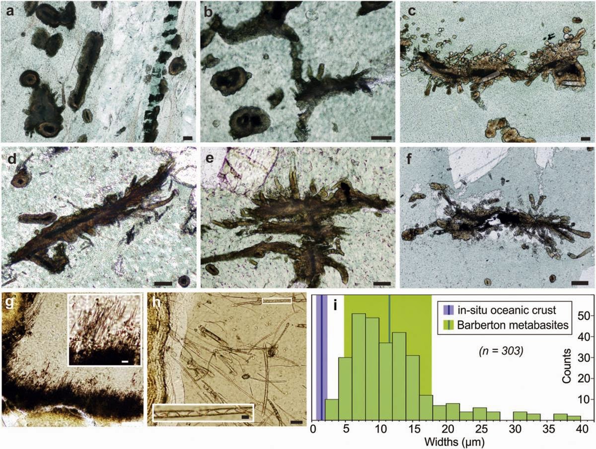
In the hunt for early life, geobiologists seek evidence of ancient microbes in the form of trace fossils – geological records of biological activity – embedded in lavas beneath the ocean floor. Filamentous titanite (a calcium titanium silicate mineral) microtextures found in 3.45 billion-year-old volcanic pillow lavas of the Barberton greenstone belt of South Africa, have been argued previously2 to be Earth’s oldest trace fossil, representing the mineralized remains of microbial tunnels in seafloor volcanic glass. However, scientists at the University of Bergen, Norway have reported new data based on in situ U-Pb (uranium-lead) dating, metamorphic temperature mapping constraints and morphological observations that bring the biological origin of these fossils into serious question.
The new age determined for the titanite microtextures is much younger than the eruptive and seafloor hydrothermal age of the previously proposed bioalteration model. As a result, the researchers have analyzed these fossils’ syngenicity (age as estimated by a textural, chemical, mineral, or biological feature formed at the same time as its encapsulating material) and biogenicity (any chemical and/or morphological signature preserved over a range of spatial scales in rocks, minerals, ice, or dust particles that are uniquely produced by past or present organisms). The scientists conclude that the oldest bona fide biogenic trace fossil now reverts to roughly 1.7 Ga microborings in silicified stromatolites found in China, and that the search for subsurface life – both on the early Earth as well as in extraterrestrial mafic–ultramafic rocks1, such as Martian basalts – be based not only on new biosignatures, but on new detection techniques as well.
Dr. Eugene G. Grosch discussed the paper that he and Dr. Nicola McLoughlin published in Proceedings of the National Academy of Sciences. “Previous work2 argued that titanite formed inside, or infilled, hollow tubes initially proposed to have been made by microbes living in the volcanic subseafloor at around 3.472 billion years ago – but the age estimate of the trace fossil formation and mineralization was not well constrained,” Grosch tells Phys.org. “In our PNAS study we took a critical approach, conducting a syngenicity test of the previous bioalteration model to determine if the titanite did indeed form 3.472 billion years ago during subseafloor hydrothermal alteration and Paleoarchean glass microbial bioalteration.” Using two laser-ablation inductively coupled plasma mass spectrometry, or LA-ICP-MS, instruments (single- and multi-collector), and a uranium-to-lead isotopic decay radiometric system, the scientists dated the titanite at roughly 2.9 billion years old – too recent for the titanite to be syngenetic with the 3.472 billion year old bioalteration model. “This was a challenge,” Grosch adds, “because these rocks are extremely old, so we had to be careful to take into account common lead in the titanite mineral.”
In order to potentially make a claim or confirm earliest candidate traces of life in Archean subseafloor environments, the researchers propose that careful geological work should first be conducted and that low-temperature metamorphic events should be completely characterized in Archean greenstone belt pillow lavas (bulbous, spherical, or tubular lobes of lava attributed to subaqueous extrusion). They accomplished this by using a new quantitative electron microprobe microscale mapping technique to map the composition of different minerals associated with the putative titanite filaments. In addition, they applied an inverse thermodynamic modelling approach to the mineral chlorite in the maps and calculated a metamorphic temperature map in the matrix surrounding a candidate titanite trace fossil. Their results showed, for the first time, constraints on metamorphic conditions and that on a microscopic scale, the best-developed titanite filaments were associated with the low-temperature microdomains. “This discovery indicates a cooling history around the titanite filaments, and supports an abiotic – that is, not associated with life – mineral growth mechanism at 2.9 Ga,” Grosch explains. “This proves that the titanite was a result of much younger metamorphic growth and not related to the posited biological activity in the 3.472 Ga bioalteration model constructed by previous investigators. Moreover, filamentous titanite cannot be used as a biosignature because it has failed a wide range of syngenicity and biogenicity tests.”
Finding that these titanite microtextures exhibit a morphological continuum bearing no similarity to candidate biotextures found in the modern oceanic crust also supports their conclusions. “One of the main lines of evidence in our study that questions the biogenicity of the titanite microtextures is the huge range of shapes and sizes that they exhibit,” Grosch tells Phys.org. “This contradicts the general principle accepted by palaeontologists that a fossil population should show a restricted size distribution that reflects biological control on growth, as opposed to self-organizing abiotic processes that do not show restricted size distributions. Furthermore, we argue that the growth continuum in the Barberton titanite microtextures, from oval-shaped hornfelsic (thermally metamorphosed rock) structures with few projections to coalesced oval-shaped structures that progress into bands with increasing number and size of filamentous projections, records an abiotic, metamorphic growth process and not the earlier seafloor trace fossil model. Lastly, in contrast to the microtextures of argued biogenic origin from the modern oceanic crust which do show a narrow size distribution and specific shapes, the Barberton microtextures show a much greater range in sizes – at least an order of magnitude greater – and a much larger spectrum of morphologies.”
To address the challenges encountered in their research, Grosch says that the key insight was that all the tests and in situ data indicated that titanite microtextures failed as a biosignature that represents Earth’s oldest trace fossil. “In addition,” he notes, “there are no organics such as decayed carbon or nitrogen associated with the titanite; the size, shape and distribution of the filamentous titanite are all not compatible with that expected for a biogenic population; the age is much too young at 2.8-2.9 billion years ago; and the quantitative petrological mapping indicates a thermal history compatible with an abiotic growth of titanite filaments, not as infilling minerals as previous studies have proposed.” (Petrology is the branch of geology that studies the origin, composition, distribution and structure of rocks.). Grosch concludes that filamentous titanite microtextures, such as those in the Barberton pillow lavas, can no longer be used as a biological search image for life in Archean metavolcanic glass, and that other search images combined with morphological and biogeochemical evidence for early life need to be found. “If we want to make a robust case for early life preserved in Archean volcanic rocks or any other ancient rock, we need to look for early morphological and biogeochemical biosignatures – but we also have to combine these with high-resolution 2- and 3-dimensional mapping and reconstructions,” he points out. “We also need to prove a ‘fossil’ is a very early structure preserved in the rock and not a later abiotic feature. We need to find new ways to carefully peel back layers of deep geological time and eliminate all abiotic scenarios first before we can be sure of an early body or trace fossil.”
Regarding biogeochemical traces of life on early Earth, the scientists have found that the sulfur isotopes of microscopic sulfide minerals found in the Barberton pillow lavas have unusually large fractionations (the ratio of light to heavy 32 to 34 sulfur atoms), and that this could record the activities of sulfur-based microbes in the Archean subseafloor. “In a previous study led by co-author Dr. Nicola McLoughlin3,” Grosch continues, “we suggested that these types of chemical signatures need to be further investigated as possible alternative evidence for an early subseafloor biosphere on early Earth. Such signatures are known from ancient sediments, where they are widely accepted as evidence of early sulfur based life forms – but this was the first and earliest evidence from subseafloor volcanic rocks.” In a previous work3, the scientists state that alternatives such as sulfur isotope fractionations recorded by basalt-hosted sulfides could be more promising in the search for evidence of ancient life. Grosch notes that today’s microbes use the light isotope in their metabolic pathways, such as 32S in microbial sulfate reduction. As a consequence, when seawater sulfate is used for energy by these microbes, the mineral pyrite, or FeS2, is formed as a reaction byproduct. As such, the fraction in the sulfur 32S/34 S ratio is large and can therefore be measured in the FeS2. “We can measure the pyrite 32S/34S ratio relative to an international standard derived from meteoritic sulfide and use the degree of fractionation as a biogeochemical marker. That’s a wide range of 32/34S ratios – and a negative range is a good geochemical sign of possible early Archean microbial life.”
Grosch also discusses the prospect of looking for signs of early life in extraterrestrial mafic-ultramafic rocks by adopting a highly critical and multi-pronged analytical testing approach towards biogenicity. “Until one day in the future when space missions return samples from Mars, we have to use satellite-based remote sensing techniques to investigate the abundant mafic-ultramafic rocks found on Mars.” (He adds that Martian meteorites are also of interest – particularly a group called Nakhalites that contain igneous minerals and are believed to show evidence of aqueous alteration and possible biosignatures) A good strategy,” he says, “would be to focus on locations where there’s strong evidence for water-rock interaction and preserved organic carbon, because these sites may have chemical gradients that could help sustain microbes.” In fact, in another study4 the scientists explore how microscale mapping of the low-temperature minerals in such rocks could be used to investigate their alteration history and to evaluate the possibility of preserving chemical and textural traces of life in extra-terrestrial mafic-ultramafic rocks.
“We need to look carefully for possible microbe morphologies and possible preserved microbial activity in extraterrestrial samples. We need to apply new thermodynamic and high-resolution analytical petrological techniques such as metamorphic, nano-SIMS and soft X-ray (synchrotron) mapping techniques to understand very low-temperature conditions of hydrothermal alteration and possible signs and preservation of microbial life in samples from other rocky planets, such as Mars.”
Moving forward, Grosch identifies the key next steps in their research and other possible innovations:
Extensive geological mapping of the Barberton Greenstone Belt, South Africa to identify alternative locations and evidence for early microbial life
Further studies of recent seafloor volcanic glass to establish if the microtunnels are really the product of microbial life – and if so, what type of microorganisms are involved
Further geochronological work – that is, radiometric dating to better establish the timing of geological events and age of different environments in these ancient Archean rocks
Development and refinement of thermodynamic models, in metamorphic petrology tools and in situ geochemistry techniques to better characterize and test microscopic textural and chemical evidence of putative life in Archean rocks
Apply and compare multiple high-resolution techniques to candidate biosignatures in ancient rocks
Grosch notes that there are other areas of research that might benefit from their study. “In the field of paleontology, fossil experts now need to go and look for the oldest robust trace fossils – and while that our study questions the evidence in ancient metamorphic pillow lavas, and that the oldest bona fide candidate trace fossil comes from 1.7 billion year old rocks in China, if paleontologists look harder and in the right places, they may find trace fossils and evidence of microbial activities in older rocks, such as silicified seafloor sediments or in shallow marine Archean environments. In addition, from our findings we propose to astrobiologists and planetary scientists that looking for filamentous titanite microtextures as an extraterrestrial biosignature is misleading, and therefore they should seek other evidence for subsurface life on other wet rocky planets in our solar system – especially Mars – and possibly beyond.”
More information:
Reassessing the biogenicity of Earth’s oldest trace fossil with implications for biosignatures in the search for early life, Proceedings of the National Academy of Sciences, Published online before print on May 27, 2014, doi:10.1073/pnas.1402565111
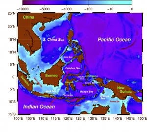
The passageway that links the Pacific Ocean to the Indian Ocean
The passageway that links the Pacific Ocean to the Indian Ocean is acting differently because of climate change, and now its new behavior could, in turn, affect climate in both ocean basins in new ways.
UH Mānoa physical oceanographer James Potemra is co-author of a study led by Janet Sprintall of Scripps Institution of Oceanography at UC San Diego. The scientists have found that the flow of water in the Indonesian Throughflow – the network of straits that pass Indonesia’s islands – has changed since the late 2000s under the influence of dominant La Niña conditions. The flow has become more shallow and intense in the manner that water flows through a hose that has become kinked. The study suggests that human-caused climate change might make this characteristic a more dominant feature of the throughflow, even when El Niño conditions return.
Sprintall and colleagues have spent more than a decade understanding the dynamics of the throughflow, an ocean region that acts like a cable sending information between two electronic devices. The Indonesian seas are the only tropical location in the world where two oceans interact in this manner. The throughflow has an effect on the climate well beyond its boundaries, playing a role in everything from Indian monsoons to the El Niño phenomena experienced by California.
“This is a seminal paper on a key oceanographic feature that may have great utility in climate research in this century,” said Eric Lindstrom, a physical oceanography program scientist who co-chairs the Global Ocean Observing System Steering Committee at NASA, which funded Sprintall’s portion of the study. “The connection of the Pacific and Indian oceans through the Indonesian Seas is modulated by a complex circulation, climate variations, and sensitive ocean-atmosphere feedbacks. It’s a great place for us to sustain ocean observations to monitor potential changes in the ocean’s general circulation under a changing climate.”
Sprintall, a physical oceanographer at Scripps Oceanography, said this new research starts a new chapter in the history of the throughflow, one characterized by the changed variables created by global warming.
“Now that we have a better understanding of how the Indonesian Throughflow responds to El Niño and La Niña variability, we can begin to understand how this current behaves in response to changes in the trade wind system that are brought on through anthropogenic climate change,” Sprintall said. “Changes in the amount of warm water that is carried by the throughflow will have a subsequent impact on the sea surface temperature and so shift the patterns of rainfall in the whole Asian region.”
The study, “The Indonesian seas and their role in the coupled ocean-climate system,” appeared in the June 22 advance online publication of the journal Nature Geoscience.
In previous work over the past decade, Sprintall and colleagues from several countries have revised earlier thinking that most of the action in the throughflow was just at the surface where winds and waves interact. In fact, the flow often runs as much as 100 meters (328 feet) below the surface and features upwellings and other strong vertical flows of water. Model simulations have suggested that without this flow, the Indian Ocean would be generally colder at the surface as the Pacific would not be able to route warm water to it as efficiently.
These computer-generated scenarios have helped researchers forecast what could be happening as a consequence of human-caused climate change. Since the mid-twentieth century, scientists have noticed that Pacific Ocean tradewinds are weakening. The tradewinds help push Pacific Ocean water toward the throughflow and ultimately to the Indian Ocean. This corresponds to a predicted general slowdown of global thermohaline circulation – the flow of heat and salt around the world’s oceans.
The researchers found that as a strong El Niño regime begun in the late 1990s slowly yielded to La Niña conditions in the middle of the following decade, the nature of the throughflow changed. The strongest currents became shallower and faster through the main component of the throughflow, the Makassar Strait that runs between the Indonesian islands of Kalimantan and Sulawesi.
La Niña and El Niño are characterized in part by the location of a warm pool of surface water in the Pacific Ocean. Warm water in the western Pacific near Indonesia is usually associated with La Niña and warm water in the eastern equatorial Pacific with El Niño.
The researchers said the study provides an important consideration that should guide the intense marine conservation efforts that are underway in Indonesia and neighboring countries. The nature of the throughflow has a direct influence on what nutrients get delivered to marine organisms in the region and in what quantity. The work also suggests that ongoing regular observations of what is happening in the throughflow are a necessity going forward.
More information:
“The Indonesian seas and their role in the coupled ocean–climate system.” Janet Sprintall, et al. Nature Geoscience (2014) DOI: 10.1038/ngeo2188. Received 02 January 2014 Accepted 21 May 2014 Published online 22 June 2014
Note : The above story is based on materials provided by University of Hawaii at Manoa
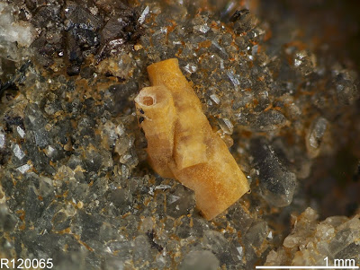
Chemical Formula: Ca(Ce,La)2(CO3)3F2 Locality: Emerald mines, Muso, columbia. Name Origin: Named for J. J. Paris, mine proprietor at Muzo, north of Bogota, Columbia.
Parisite is a rare mineral consisting of cerium, lanthanum and calcium fluoro-carbonate, Ca(Ce,La)2(CO3)3F2. Parisite is mostly parisite-(Ce), but when neodymium is present in the structure the mineral becomes parisite-(Nd).
It is found only as crystals, which belong to the trigonal or monoclinic pseudo-hexagonal system and usually have the form of acute double pyramids terminated by the basal planes; the faces of the hexagonal pyramids are striated horizontally, and parallel to the basal plane there is a perfect cleavage. The crystals are hair-brown in color and are translucent. The hardness is 4.5 and the specific gravity is 4.36. Light which has traversed a crystal of parisite exhibits a characteristic absorption spectrum.
At first, the only known occurrence of this mineral was in the famous emerald mine at Muzo in Colombia, South America, where it was found by J.J. Paris, who rediscovered and worked the mine in the early part of the 19th century; here it is associated with emerald in a bituminous limestone of Cretaceous age.
Closely allied to parisite, and indeed first described as such, is a mineral from the nepheline-syenite district of Julianehaab in south Greenland. To this the name synchysite has been given. The crystals are rhombohedral (as distinct from hexagonal; they have the composition CeFCa(CO3)2, and specific gravity of 2.90. At the same locality there is also found a barium-parisite, which differs from the Colombian parisite in containing barium in place of calcium, the formula being (CeF)2Ba(CO3)3: this is named cordylite on account of the club-shaped form of its hexagonal crystals. Bastnasite is a cerium lanthanum and neodymium fluoro-carbonate (CeF)CO3, from Bastnas, near Riddarhyttan, in Vestmanland, Sweden, and the Pikes Peak region in Colorado, U.S.A.
History
Discovery date : 1845 Town of Origin: DISTRICT DE MUZO, BOGOTA Country of Origin : COLOMBIE
Physical properties
Hardnes : 4,50 Density : 4,36 Color : brownish yellow; brown; yellow; grayish yellow Luster: vitreous; resinous; nacreous Streak : white Break : sub-conchoidal; splintery Cleavage : Yes
Photos :
Parisite-(Ce) Muzo Mine, Boyaca Department, Colombia (TYPE LOCALITY) Small Cabinet, 6.3 x 5.0 x 3.5 cm “Courtesy of Rob Lavinsky, The Arkenstone, www.iRocks.com”
A collaborative research team has discovered an important link between the eruption of Earth’s hottest lavas, the location of some of the largest ore deposits and the emergence of the first land masses on the planet – the continents – more than 2500 million years ago.
The research team includes researchers from the Centre for Exploration Targeting at The University of Western Australia and Curtin University, which are key nodes of the ARC Centre of Excellence for Core to Crust Fluid Systems, in collaboration with colleagues from CSIRO and the Geological Survey of Western Australia.
The generation and evolution of the Earth’s continental crust has played a fundamental role in the development of the planet. Its formation modified the composition of the Earth’s interior, contributed to the establishment of the atmosphere and led to the creation of ecological niches, essential for early life.
The study, published today in the prestigious international journal Proceedings of the National Academy of Sciences, used a combination of different radiogenic isotopes to show that in the early evolutionary stages of our planet, the formation and stabilisation of continents also controlled the location and extent of major komatiite volcanic eruptions.
Study co-author Professor Marco Fiorentini said komatiites were ultra-high temperature lavas that erupted in large volumes more than 2500 million years ago (Archean eon), but only very rarely since.
“They are the signature rock type of a hotter Earth in the primordial stages of its evolution, and provide the most direct link between the Earth’s interior and the Earth’s surface,” Professor Fiorentini said.
“They locally contain some of the largest known deposits of metals such as nickel, cobalt and platinum. Due to the unique geological processes that led to the formation of komatiites, they represent a rare window into the development of the innermost parts of our planet, notably the deep and inaccessible mantle and core.”
Focusing on the Yilgarn Craton of Western Australia as a natural laboratory, the research team combined sophisticated geochemical and isotopic techniques to unveil the progressive development of an Archean micro-continent.
Results from this study show that in the ancient Earth, relatively small crustal ‘blocks’, not unlike modern micro-plates, progressively developed and coalesced to form larger continental masses, called cratons, Professor Fiorentini said.
“This ‘cratonisation’ process formed deep roots to the continental land masses, extending more than 200km deep into the Earth,” he said. “The roots drove the hottest and most voluminous komatiite eruptions to the edge of established continental blocks. The ability to map these continental blocks through time points to the location where major metal deposits formed in these lavas.”
As a result, the dynamic evolution of the early continents directly influenced where deep mantle material was added to the Archean crust, oceans and atmosphere.
The complex interaction between the eruptions of some of the hottest lavas that ever existed on the planet, with the emergence of the first continents, provided a fundamental control on the distribution of major ore deposits. It also had an irreversible impact on the nature of the terrestrial biosphere-hydrosphere-atmosphere.
Reference:
David R. Mole, Marco L. Fiorentini, Nicolas Thebaud, Kevin F. Cassidy, T. Campbell McCuaig, Christopher L. Kirkland, Sandra S. Romano, Michael P. Doublier, Elena A. Belousova, Stephen J. Barnes, and John Miller. “Archean komatiite volcanism controlled by the evolution of early continents.” PNAS 2014 ; published ahead of print June 23, 2014, DOI: 10.1073/pnas.1400273111
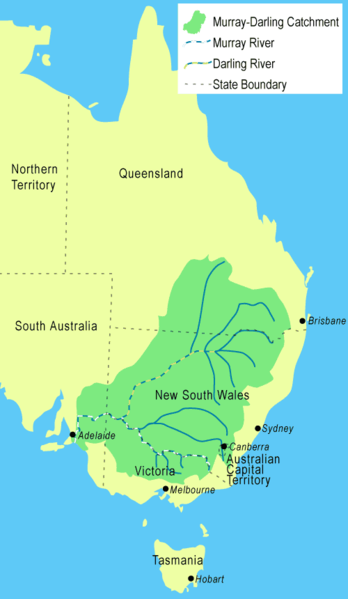
The Darling River is the third longest river in Australia, measuring 1,472 kilometres (915 mi) from its source in northern New South Wales to its confluence with the Murray River at Wentworth, New South Wales. Including its longest contiguous tributaries it is 2,844 km (1,767 mi) long, making it the longest river system in Australia.
The Darling River is the outback’s most famous waterway. The Darling has been in poor health, suffering from overuse of its waters, pollution from pesticide runoff and prolonged drought. In some years it has barely flowed at all. The river has a high salt content and declining water quality. Increased rainfall in its catchment in 2010 has improved flow, but the health of the river will depend on long-term management.
The Division of Darling, Division of Riverina-Darling, Electoral district of Darling and Electoral district of Lachlan and Lower Darling were named after the river.
History
The Queensland headwaters of the Darling (the area now known as the Darling Downs) were gradually colonised from 1815 onward. In 1828 the explorer Charles Sturt and Hamilton Hume were sent by the Governor of New South Wales, Sir Ralph Darling, to investigate the course of the Macquarie River. He discovered the Bogan River and then, early in 1829, the upper Darling, which he named after the Governor. In 1835, Major Thomas Mitchell travelled a 483 km portion of the Darling River. Although his party never reached the junction with the Murray River he correctly assumed the rivers joined.
In 1856, the Blandowski Expedition set off for the junction of the Darling and Murray Rivers to discover and collect fish species for the National Museum. The expedition was a success with 17,400 specimens arriving in Adelaide the next year.
Although its flow is extraordinarily irregular (the river dried up on no fewer than forty-five occasions between 1885 and 1960), in the later 19th century the Darling became a major transportation route, the pastoralists of western New South Wales using it to send their wool by shallow-draft paddle steamer from busy river ports such as Bourke and Wilcannia to the South Australian railheads at Morgan and Murray Bridge. But over the past century the river’s importance as a transportation route has declined.
In 1992, the Darling River suffered from severe cyanobacterial bloom that stretched the length of the river.The presence of phosphorus was essential for the toxic algae to flourish. Flow rates, turbulence, turbidity and temperature were other contributing factors.
In 2008, the Federal government spent $23 million to buy Toorale Station in northern New South Wales, which allowed for the return of eleven gigalitres of environmental flows.
Course
The whole Murray-Darling river system, one of the largest in the world, drains all of New South Wales west of the Great Dividing Range, much of northern Victoria and southern Queensland and parts of South Australia. Its meandering course is three times longer than the direct distance it traverses.
Much of the land that the Darling flows through are plains and is therefore relatively flat, having an average gradient of just 16 mm per kilometre. Officially the Darling begins between Brewarrina and Bourke at the confluence of the Culgoa and Barwon rivers; streams whose tributaries rise in the ranges of southern Queensland and northern New South Wales west of the Great Dividing Range. These tributaries include the Balonne River (of which the Culgoa is one of three main branches) and its tributaries; the Macintyre River and its tributaries such as the Dumaresq River and the Severn Rivers (there are two – one either side or the state border); the Gwydir River; the Namoi River; the Castlereagh River; and the Macquarie River. Other rivers join the Darling near Bourke or below – the Bogan River, the Warrego River and Paroo River.
Darling River at Louth
South east of Broken Hill, the Menindee Lakes are a series of lakes that were once connected to the Darling River by short creeks. The Menindee Lake Scheme has reduced the frequency of flooding in the Menindee Lakes. As a result about 13,800 hectares of lignum and 8,700 hectares of Black box have been destroyed. Weirs and constant low flows have fragmented the river system and blocked fish passage.
The Darling River runs south-south-west, leaving the Far West region of New South Wales, to join the Murray River on the New South Wales – Victoria border at Wentworth, New South Wales.
The Barrier Highway at Wilcania, the Silver City Highway at Wentworth and the Broken Hill railway line at Medindee, all cross the Darling River. Part of the river north of Menindee marks the border of Kinchega National Park. In response to the 1956 Murray River flood a weir was constructed at Menindee to mitigate flows from the Darling River.
The north of the Darling River is in the Southeast Australia temperate savanna ecoregion and the south west of the Darling is part of the Murray Darling Depression ecoregion.
Population centres
Major settlements along the river include Brewarrina, Bourke, Louth, Tilpa, Wilcannia, Menindee, Pooncarie and Wentworth. Wentworth was Australia’s busiest inland port in the late 1880s.
Navigation by steam boat to Brewarrina was first achieved in 1859. Brewarrina was also the location of inter-tribal meetings for Indigenous Australians who speak Darling and live in the river basin. Ancient fish traps in the river provided food for feasts. These heritage listed rock formations have been estimated at more than 40,000 years old making them the oldest man-made structure on the planet.
Note : The above story is based on materials provided by Wikipedia
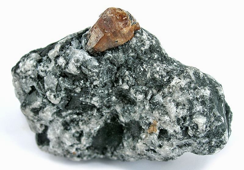
Chemical Formula: Fe2+Al2(PO4)2(OH)2·8H2O Locality: Llallagua, Potosi, Bolivia. Name Origin: Named for the chemical similarity to vauxite. Polymorph of metavauxite.
History
Discovery date : 1922 Town of Origin: LLALLAGUA, POTOSI Country of Origin : BOLIVIE
Optical properties
Optical and misc. Properties : Transparent – Translucide – Fragile, cassant Refractive Index : from 1,55 to 1,57 Axial angle 2V: 72°
Physical properties
Hardness: 3,00 Density : 2,36 Color : colorless; greenish white Luster : vitreous; nacreous Streak: white Break: conchoidal Cleavage : Yes
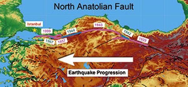
Earthquake progression with time along the North Anatolian Fault.
Is one of the world’s great cities due to be struck by a serious earthquake? Ekbal Hussain describes how scientists are working to make sure Istanbul is prepared for the dangers that may be on the way.
Straddling the European and Asian borders Istanbul is an ancient and beautiful city. Once known as Constantinople, it has been at the centre of major empires including the Roman, Byzantine, Latin and Ottoman. This great city is inundated with rich culture and history, and with nearly 14 million inhabitants it is also one of the largest cities in the world.
But this thriving metropolis sits on the edge of one of the fastest moving faults in the world: the North Anatolian Fault. This is a system of large fractures within the Earth on which energy, from the motion of the tectonic plates, is stored and released in earthquakes.
The North Anatolian Fault is roughly 1300km long, running along the entire length of northern Turkey from the Aegean Sea in the west to Lake Van in the east. It slips such that central and southern Turkey are moving west relative to northern Turkey at speeds of 20-30mm a year. It is the most active and destructive earthquake-prone fault system in Turkey.
It has been known for a while now that earthquakes on the fault tend to follow a regular sequence. That is, an earthquake will often occur on the section of the fault adjacent to the last rupture. Starting with the 1939 magnitude 7.9 Erzincan earthquake and culminating in the 1999 magnitude 7.4 and 7.2 earthquakes, there have been 12 events with magnitudes greater than 6.4 that together have ruptured almost the entire length of the fault.
The map shows this westward progression of seismic activity. The 1999 Izmit (magnitude 7.4) and Duzce (magnitude 7.2) earthquakes killed about 18,000 people, mostly in the city of Izmit. These events occurred less than 100km east of Istanbul, leading some researchers to predict the next quake will strike Istanbul itself.
Seismologists calculate the chance of an earthquake greater than magnitude 7 occurring near Istanbul in the next 30 years at somewhere between 35 and 70 per cent. And with almost a million people moving to the metropolis every year it is no surprise that Istanbul is a major candidate for the so called ‘million-death quake.’
We need to improve our ability to forecast such quakes by creating realistic models of the fault’s behaviour, and to do this we need to know more about the fault itself.
The NERC-funded FaultLab project based at the University of Leeds is helping address these problems, with support from the University’s Climate and Geohazard Services group. The investigators use data from a multitude of sources including satellite radar and geological observations, as well as data from the densest network of seismic stations ever deployed across a fault.
The project scientists aim to use the seismic data to investigate the deep structure of the fault and to see if there are differences in the crust either side of the fracture. The geologists will be looking at an old fault zone to probe the microscopic structure of minerals inside these large fracture zones. Together, these observations will enable us to better understand what the fault is doing deep in the ground and how this has affected the crust adjacent to it. The geodesy group (earth observation scientists) will use satellite radar to make accurate maps of how the ground surface is moving and relate that to the amount of energy being stored on the fault. Finally, the modelling team will link these observations together to produce an accurate picture of the behaviour of the fault. These results can then feed into models to make a more realistic forecast of the hazard Istanbul faces.
A resilient city
Professor Nicholas Ambraseys, a leading expert in the field, famously said: ‘Earthquakes don’t kill people, buildings do.’
We technically don’t need to know when the earthquake will occur to save lives. Death and injury can be prevented through simple engineering works to reinforce vulnerable buildings and by ensuring new structures are built to earthquake-resilient standards. It’s estimated to cost only 10 per cent more to build a house that is earthquake resistant compared to one that isn’t.
The Turkish government has not been idle. The new Sabiha Gökçen International Airport terminal, which opened in October 2009, is designed to withstand shaking from a magnitude 8 earthquake and, importantly, keep working afterwards – this will be an important entry point for foreign aid after a disaster.
The Marmaray rail tunnel, opened in October 2013, runs beneath the Bosphorus Straits and links the European and Asian sides of the country. The rail tunnel was built to withstand a magnitude 9 earthquake.
In May 2012 a new Urban Transformation Law was passed, stating that all buildings that do not meet current earthquake hazard criteria will be demolished. This means nearly 6.5 million buildings throughout Turkey could be demolished over the next two decades, and will pave the way for more resilient cities.
Ambitions on this scale need strong governance and management, but they also need good science – to help the Turkish government prioritise its engineering projects and work on effective evacuation and mitigation plans. The results from the FaultLab project will help develop and refine their forecast models, so those plans can be put in action the moment there’s a sign that a deadly earthquake is imminent.
Last week, scientists reported finding rocks made of plastic on a Hawaiian beach. Some researchers have speculated that these and other humanmade objects could become part of the fossil record, defining a human-dominated period of Earth’s history called the Anthropocene. Science chatted with Jan Zalasiewicz, a paleontologist at the University of Leicester in the United Kingdom and a leading scholar on the Anthropocene, about the kinds of things humans are leaving behind—and what they’ll look like millions of years hence.
This interview has been edited for clarity and brevity.
Q: You have called these humanmade fossils “technofossils.” What are they, and how are they different from normal fossils?
A: Technofossils are basically all the things we manufacture, large and small. Because most of them are preservable, they can potentially become fossils—particularly since, unlike nature, we’re so poor at recycling the things we make. They can survive for thousands, millions, perhaps billions of years in rock strata [rock or sediment layers] in the future. We think they deserve a separate category because there’s so much about them that is distinct.
Q: What kinds of things can we expect to survive in the fossil record for millions of years, and what will they look like after all that time?
A: Looking around at my room, I’m struggling to see anything that is not fossilizable. So let’s take my desk—wood can fossilize really quite well. We’ve helped along the process of fossilization of this wood because it’s been seasoned, dried out, and varnished. It’s much less edible than it was in its original state on the tree.
With clothes, a lot of them are made from plastic polymer objects or cotton—plant materials. So they will fossilize just as plants do. They can preserve a good deal of the fabric. Under the right circumstances, one can preserve leaf cells and the like for millions of years—but the chemistry will change, they will become carbonized. You will lose the colors, and they’ll become black shapes.
Even paper is fossilizable. Now clearly, if that makes it into a stratum, it will become a carbonized lump. Probably the information on the pages is not easily fossilizable. It would be very hard to read newsprint from pages.
This computer I have in front of me, I see plastic, titanium, bits of rubber, a fair bit of this—if buried in the stratum—it will at least leave a nice oblong detail and impression, probably parts of the structure itself. But the information will be gone. Just as we can fossilize a songbird, it’s much harder to fossilize the song itself.
Q: Are some cities more likely to preserve technofossils than others?
A: In San Francisco, Earth’s crust is rising. It’s being eroded and the material is being washed away to areas where the crust is subsiding. So an upland place like San Francisco will be eroded, and the fragments will wash into the sea. Los Angeles and the northwest of Britain—Manchester, say—are also on long-term upward-moving crust. These are both also destined to be eroded away.
New Orleans, in contrast, is on a delta. It’s on what’s called a tectonic escalator, going downwards because that’s what the crust is doing, and because it’s being loaded by all the sand and mud being washed off from the Mississippi River. New Orleans is ripe for fossilization, all of the structures, the pilings, the concrete pilings, tens of meters into the ground to keep the skyscrapers up. And all of the stuff that’s underground: pipework, sewage, the electric.
Other places might be Amsterdam, Venice, Shanghai, coastal deltas on coastal plains. These places are ripe for fossilization.
Q: What will future beings be able to infer about us from these fossils?
A: The technofossils will strike them as quite different as anything that’s come before. We have the whole history we see through archaeology. Metals—Bronze [Age] first, then Iron and so on, different types of tools. And then we go into the Industrial Revolution and on to the space age and beyond.
If you’re looking at the point of the perspective of the future paleontologist, either human or nonhuman or space visitor or hyperevolved rat or whatever, as a geologist one thing will strike them. will be crammed into a very small physical space. The stratum itself may not be much more than a few meters thick. In many places, it may only be a few centimeters thick. It will probably appear instantaneous, and it will be very hard work to figure out the path of this hyperevolution of the technofossils within the human stratum.
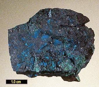
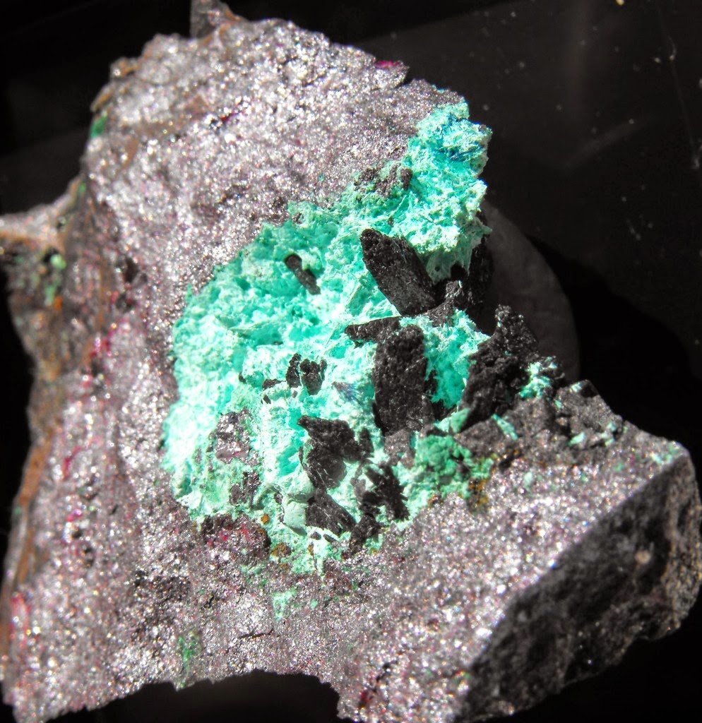
Chemical Formula: Cu2Cu2O3 Locality: Copper Queen mine, Bisbee, Arizona, USA. Name Origin: Named from the Greek for near and melaconite, which in turn was named for black and dust, now a synonym for tenorite.
Paramelaconite is a rare, black-colored copper oxide mineral with formula Cu21+Cu22+O3 (or Cu4O3). It was discovered in the Copper Queen Mine in Bisbee, Arizona, about 1890. It was described in 1892 and more fully in 1941. Its name is derived from the Greek word for “near” and the similar mineral melaconite, now known as tenorite.
Description and occurrence
Paramelaconite is black to black with a slight purple tint in color, and is white with a pinkish brown tint in reflected light. The mineral occurs with massive habit or as crystals up to 7.5 centimetres (3.0 in). A yellow color is formed when the mineral is dissolved in hydrochloric acid, a blue color when dissolved in nitric acid, and a slightly brown precipitate when exposed to ammonium hydroxide. When heated, paramelaconite breaks down into a mixture of tenorite and cuprite.
Paramelaconite is a very rare mineral; many specimens purported as such are in fact mixtures of cuprite and tenorite. Paramelaconite forms as a secondary mineral in hydrothermal deposits of copper. It occurs in association with atacamite, chrysocolla, connellite, cuprite, dioptase, goethite, malachite, plancheite, and tenorite. The mineral has been found in Cyprus, the United Kingdom, and the United States.
History
Discovery date: 1891 Town of Origin: MINE COPPER QUEEN, BISBEE, COCHISE CO., ARIZONA Country of Origin: USA
Optical properties
Optical and misc. Properties : Opaque
Physical properties
Hardness: 4,50 Density: from 6,10 to 6,11 Color : black; purplish black Luster : adamantine; bright Streak: brownish black Break: conchoidal Cleavage: NO
OUR planet is home to a glorious variety of animals, but it might not have been. Were it not for the birth pangs of a mega-continent, the evolution of animals could have stopped at its earliest stages.
We now have the best evidence yet that an enormous wave of volcanism, caused by several continents crashing together to form the even greater landmass known as Gondwana, was the reason for a sharp rise in global temperature. This change was the driving force for evolutionary explosions that made life more diverse and laid the foundations for all future animal species.
Volcanoes can cause global warming because eruptions often spew huge amounts of the greenhouse gas carbon dioxide. Now a study of volcanic rocks from early in life’s evolutionary story shows that such eruptions coincided with a change in the climate from frigid chill to sweltering heat.
This swing, and the way it affected the oceans, caused an explosion of evolutionary diversity, followed by a mass extinction when temperatures got too hot. Then, when Gondwana had formed and the volcanism died down, the planet cooled and life began to bloom again. The findings add to evidence that plate tectonics and living things are linked (see “Shaky worlds may harbour life”).
Last year, a study suggested that microbes helped form continents by encouraging volcanic activity (New Scientist, 23 November 2013, p 10). Now Ryan McKenzie of the University of Texas at Austin and colleagues have shown that, in turn, volcanism may have shaped life during the crucial Cambrian period .
Before the Cambrian, over 600 million years ago, Earth was virtually covered in ice. The first animals arose on this “Snowball Earth”, but these “Ediacarans” did not look like modern animals.
Then came the Cambrian explosion. “You had single cell organisms, single cell, single cell, then weird Ediacaran oddballs, and – suddenly – snails and bivalves and sea stars and a whole range of groups that typify the record for the rest of time,” says McKenzie’s colleague Paul Myrow of Colorado College in Colorado Springs.
The animals that appeared during the Cambrian explosion gave rise to all the major groups alive today, from worms to starfish. But each group only contained a few species, and got no further. The next period is known as the Dead Interval, and was marked by mass extinctions. It was another 50 million years before animal life blossomed once more, during the Ordovician.
We already knew that Earth’s temperature changed dramatically over these periods. It thawed in the early Cambrian then became stiflingly hot during the Dead Interval, before cooling again. “These are huge climate swings, from Snowball Earth to one of the warmest intervals of Earth history in the Cambrian,” says Lee Kump of Penn State University in University Park.
Volcanic activity during the formation of Gondwana has been suggested as a driver of these violent changes, but Kump says the evidence for increased volcanism was “a house of cards”.
McKenzie’s new evidence comes from tiny zircon crystals. Zircons are only formed in particular volcanic eruptions that are triggered when continental masses crash into each other, so they act as a record of past continental collisions. McKenzie assembled zircon counts from rocks laid down in the last 3 billion years, from all around the world.
He noticed that zircons were rare from Snowball Earth but common in the Cambrian. It seems a horde of volcanoes began spewing just before the Cambrian, and their activity reached a peak during the Dead Interval (Geology, doi.org/qvp).
“We hypothesise that CO2 outgassing from continental volcanic arcs drove major climate shifts,” says McKenzie.
Kump agrees: “This to my knowledge is the first direct and compelling assessment of changes in arc volcanism over this critical interval.”
“This is a fundamentally new and radical idea,” says Cin-ty Lee of Rice University in Houston, Texas.
Myrow says the formation of Gondwana offers the best explanation for the extra volcanoes. “Throughout the Cambrian two big continental masses were coming together to make Gondwana,” he says. The collision generated infernal heat that melted rock and created long chains of volcanoes. “You’re making volcanoes like mad,” says Myrow. “They produce carbon dioxide and temperatures get very, very hot.”
As well as heating the planet, the extra CO2 acidified the oceans. Many ocean creatures are sensitive to changes in acidity, so this could help explain the Dead Interval. Then the volcanism died off once Gondwana had formed, CO2 levels fell and a huge diversity of reef-based animals appeared.
“Now we have greater confidence that volcanism and its effect on the greenhouse gas content of the atmosphere drove climate change in deep time,” says Kump. “This had direct effects on rates of biotic diversification.”
Changes in tectonic activity would go on to affect life on Earth throughout its history, but not always in such a helpful way. For instance, almost all animal and plant life was abruptly wiped out at the end of the Permian period 251 million years ago, a time known as the Great Dying. Rapid climate change triggered by intense volcanic activity could well be to blame. Tectonics may give, but it also takes away.
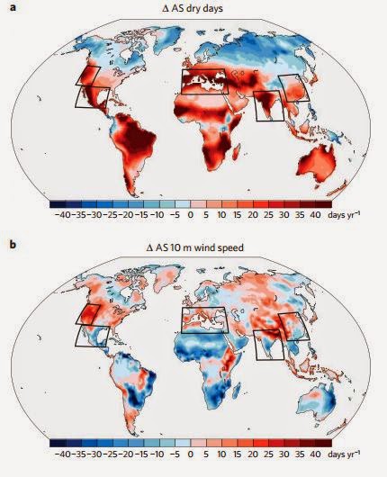
Characteristic change in air stagnation components. Credit: Nature Climate Change (2014) doi:10.1038/nclimate2272
A new study conducted by researchers at Stanford University has led to findings indicating that much of the world can expect to have more atmospheric stagnation events as the future unfolds. In their paper published in Nature Climate Change, the researchers describe how they ran a variety of computer models that took into account a continued increase in greenhouse gas emissions—they report that taken together, the models predict that approximately 55 percent of the world’s population can expect to be impacted by future stagnation events.
Stagnation is an atmospheric phenomenon where an air mass remains in place over a geographic region for an extended period of time. They tend to happen due to the convergence of specific weather conditions—light wind patterns near the surface, other light wind patterns occurring higher up, and a lack of rain. During normal weather periods, wind and rain combine to clean the air around metropolitan areas—when rain fails to fall and there is little wind to push pollution away from an area, particulates and other types of pollution levels climb, putting those that live in the area at risk of health problems.
The collection of computer models run by the team at Stanford also suggest that stagnation events are likely to last longer—increasing by an average of 40 days a year. The result the team notes, is likely to be an increase in heart and lung complications in people in those areas, contributing to an associated climb in the number of premature deaths due to air pollutants—numbering perhaps in the millions. They also note that Mexico, India and parts of the western U.S. are likely to be most at risk of health impacts from an increase in stagnation events, as all three will have more and longer such events and all three are heavily populated.
The researchers suggest that at some point, the entire planet will be impacted by stagnation events. That means governments and health workers will need to make plans on how to handle the problems as they begin to occur. They add that the only real solution to the problem is to begin curbing greenhouse gas emissions now, preventing the events from occurring in the first place.
More information: Occurrence and persistence of future atmospheric stagnation events, Nature Climate Change (2014) DOI: 10.1038/nclimate2272
Abstract
Poor air quality causes an estimated 2.6–4.4 million premature deaths per year. Hazardous conditions form when meteorological components allow the accumulation of pollutants in the near-surface atmosphere. Global-warming-driven changes to atmospheric circulation and the hydrological cycle are expected to alter the meteorological components that control pollutant build-up and dispersal, but the magnitude, direction, geographic footprint and public health impact of this alteration remain unclear. We used an air stagnation index and an ensemble of bias-corrected climate model simulations to quantify the response of stagnation occurrence and persistence to global warming. Our analysis projects increases in stagnation occurrence that cover 55% of the current global population, with areas of increase affecting ten times more people than areas of decrease. By the late twenty-first century, robust increases of up to 40 days per year are projected throughout the majority of the tropics and subtropics, as well as within isolated mid-latitude regions. Potential impacts over India, Mexico and the western US are particularly acute owing to the intersection of large populations and increases in the persistence of stagnation events, including those of extreme duration. These results indicate that anthropogenic climate change is likely to alter the level of pollutant management required to meet future air quality targets.
Chemical Formula: Zn2(AsO4)(OH) Locality: Ojuela mine, Mapimi, Durango, Mexico Name Origin: Named as the dimorph of adamite.
Paradamite is dimorphous with a famous arsenic mineral, namely adamite. Dimorphous means that the two minerals have the same formula, but different structures (di means two; morphous means shape). Paradamite’s different structure produces only slight differences in physical properties. Most obvious however is the difference in crystal forms. Adamite’s typical form is wedge shaped prismatic crystals with diamond-shaped cross-sections. Paradamite’s form is more tabular in character and very different from adamite’s. Although their names are similar and their chemistry is the same; paradamite and adamite are absolutely distinct minerals.
Optical properties
Optical and misc. Properties:Transparent Refractive Index: from 1,72 to 1,78 Axial angle 2V : 50°
Physical properties
Color : pale yellow Luster: vitreous. Transparency: Crystals are transparent to translucent. Crystal System: triclinic; bar 1.
Crystal Habits include rounded tabular crystals, usually aggregated. Cleavage: perfect. Fracture: uneven. Hardness: 3.5. Specific Gravity: approximately 4.5 – 4.6 (heavy for translucent minerals) Streak: white.
Variations in high-altitude wind patterns expose particular parts of Europe, Asia and the US to different extreme weather conditions, a new study has shown.
Changes to air flow patterns around the Northern Hemisphere are a major influence on prolonged bouts of unseasonal weather — whether it be hot, cold, wet or dry.
The high altitude winds normally blow from west to east around the planet, but do not follow a straight path. The flow meanders to the north and south, in a wave-like path.
These wave patterns are responsible for sucking either warm air from the tropics, or cold air from the Arctic, to Europe, Asia, or the US. They can also influence rainfall by steering rain-laden storms.
Pioneering new research, carried out by the University of Exeter and the University of Melbourne, has shown that the development of these wave patterns leaves certain Northern Hemisphere regions more susceptible to different types of prolonged, extreme weather.
Dr James Screen, a Mathematics Research Fellow at the University of Exeter and lead author of the study, said: “The impacts of large and slow moving atmospheric waves are different in different places. In some places amplified waves increase the chance of unusually hot conditions, and in others the risk of cold, wet or dry conditions.”
The study showed that larger waves can lead to droughts in central North America, Europe and central Asia, and western Asia exposed to prolonged wet spells. It also shows western North America and central Asia are more prone to heat waves, while eastern North America is more likely to experience prolonged outbreaks of cold.
The collaborative study used detailed land-based climate observations to identify episodes of abnormal temperature and rainfall from 1979-2012 and then examined the wave patterns during these events.
Co-author Professor Ian Simmonds, from the School of Earth Sciences at the University of Melbourne, said the weather extremes they examined were month-long heat waves, cold spells, droughts and prolonged wet periods, which occurred over large areas.
He said: “The study revealed that these types of events are strongly related to well-developed wave patterns, and that these patterns increase the chance of heat waves in western North America and central Asia, cold outbreaks in eastern North America, droughts in central North America, Europe and central Asia, and wet spells in western Asia.
“The findings are very important for decision makers in assessing the risk of, and planning for the impacts of, extreme weather events in the future.”
Note : The above story is based on materials provided by University of Exeter.