Delving into the spread of marine life: Understanding deep-sea limpets

May 29, 2014

One of Deep-sea limpets, Lepetodrilus nux. Credit: Image courtesy of OIST

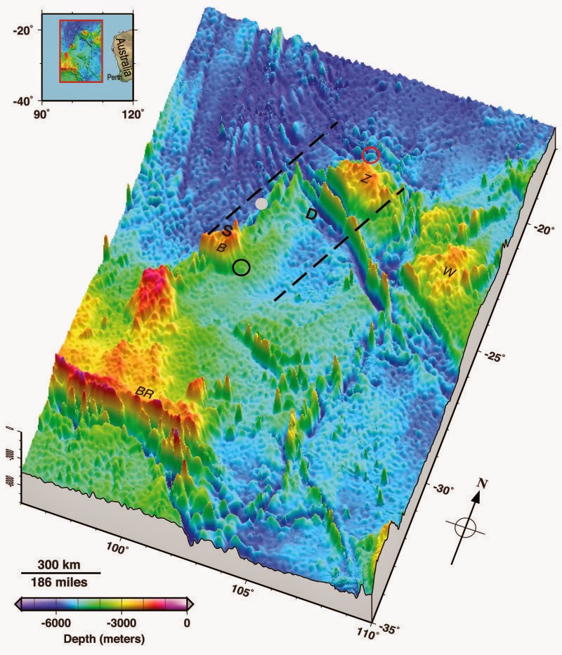
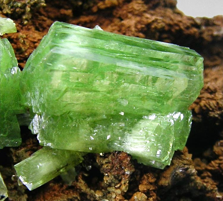
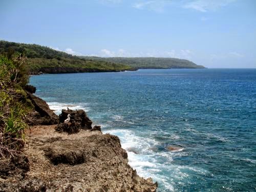
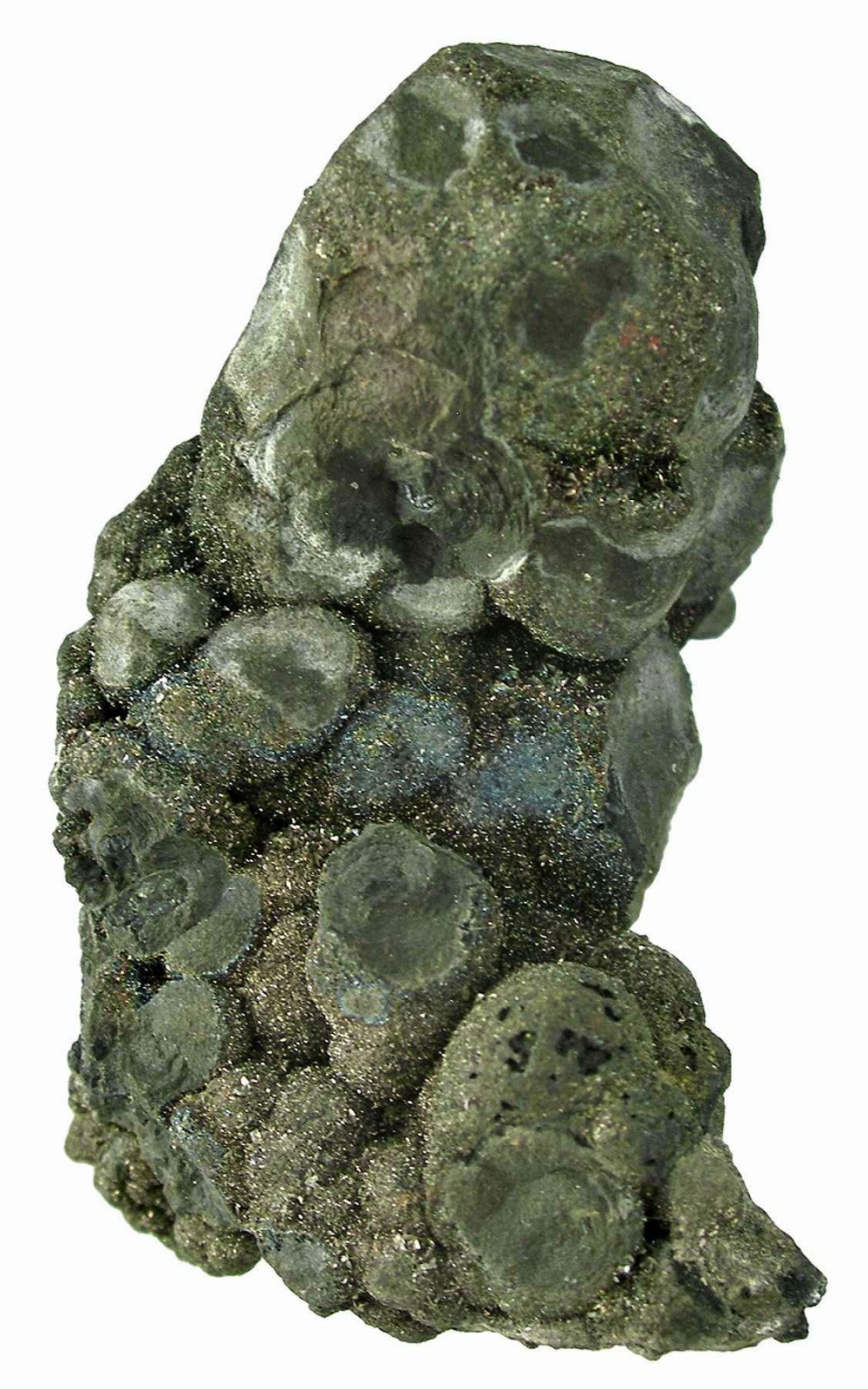
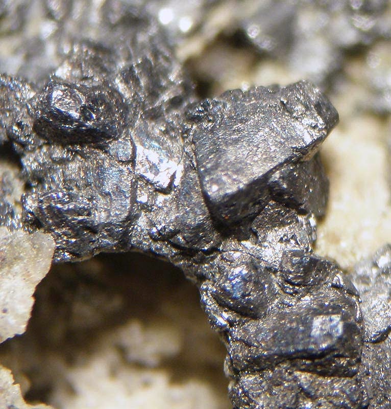
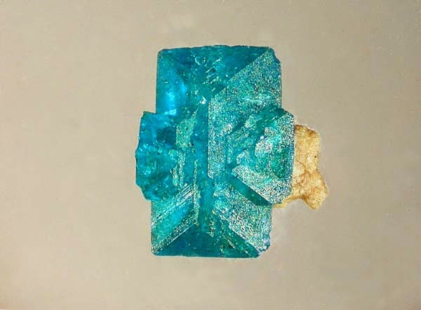
A paper by Dr. Masako Nakamura of the OIST Marine Biophysics Unit on the ecology of one of deep-sea limpets called Lepetodrilus nux has been published in the Marine Ecology Progress Series. These deep-sea limpets are conches with shells about 1 cm long. They have been confirmed to live in the long, narrow seabed known as the Okinawa Trough, located at an average of depth of 1000 meters and northwest of the Nansei and Ryukyu Islands. In this paper, three major findings are reported: new limpet habitats in the Okinawa Trough, the process of limpet population formation surmised from their shell length, and limpet reproduction patterns. This is the first study of the life history of limpets living in the Okinawa Trough, including their reproduction and spread, and Dr. Nakamura’s work provides insights into their ecological mechanisms.

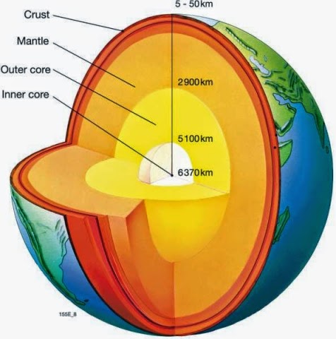
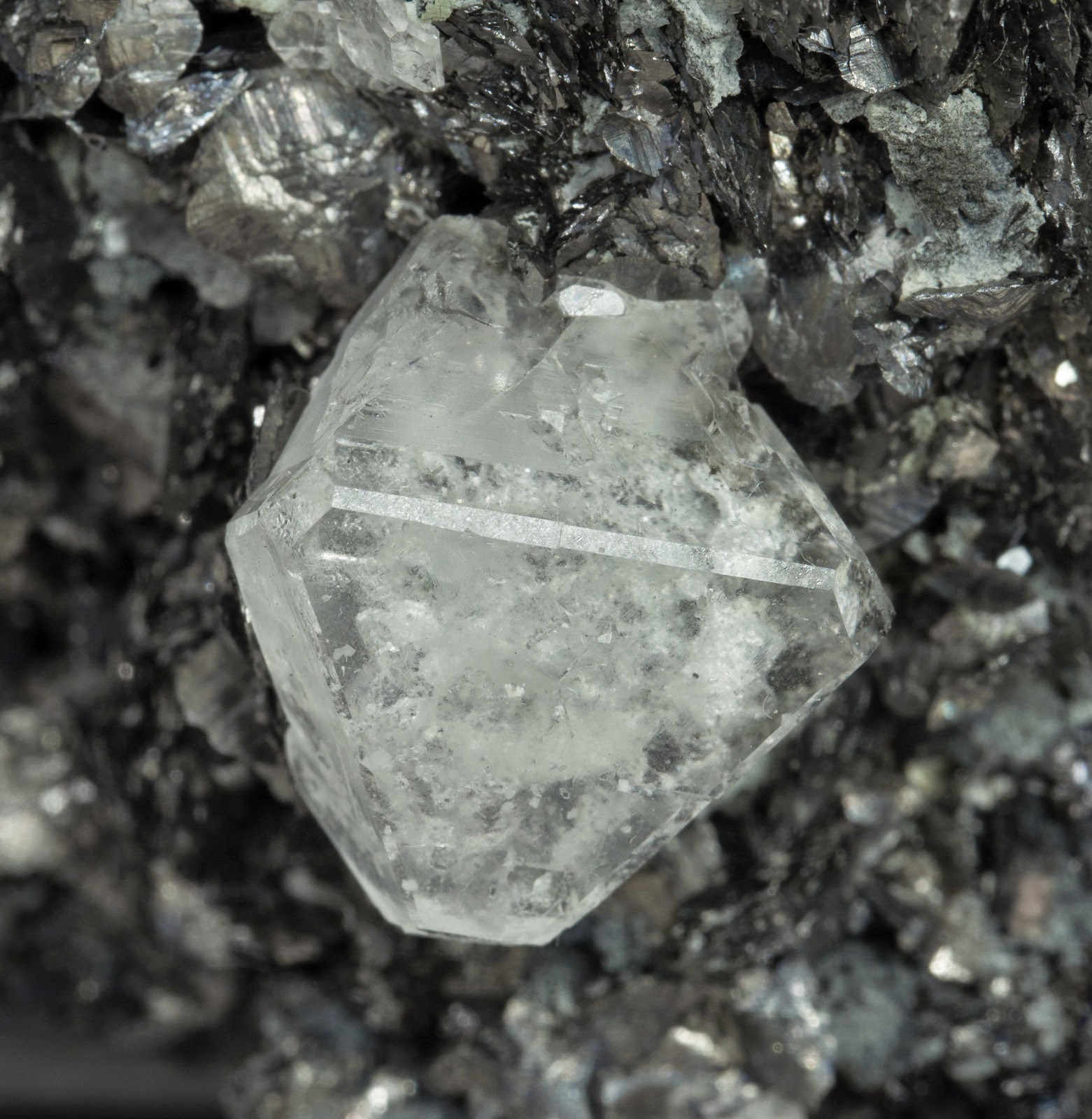
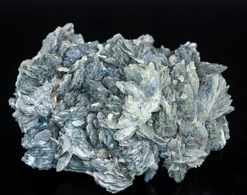
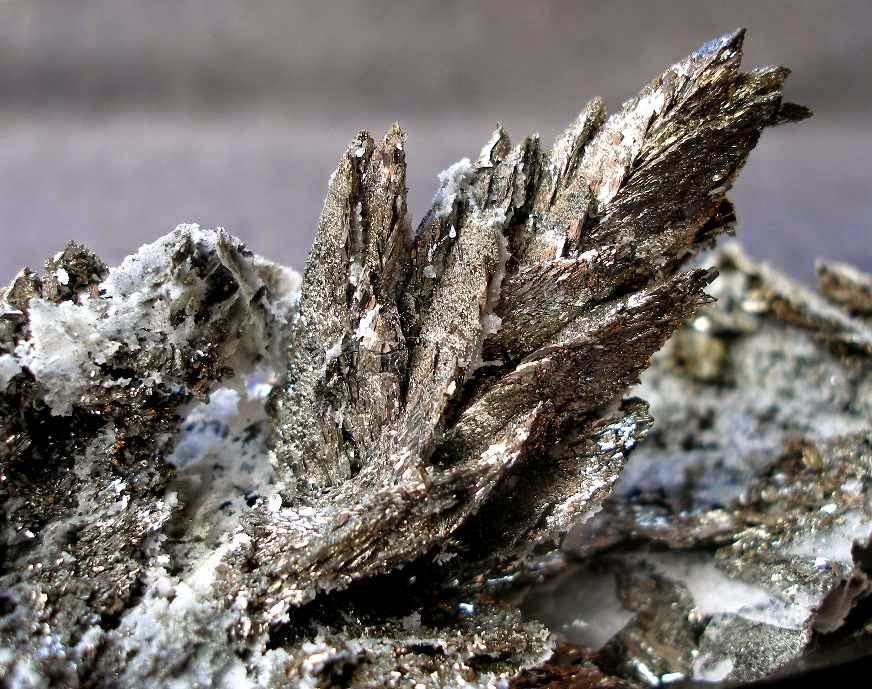
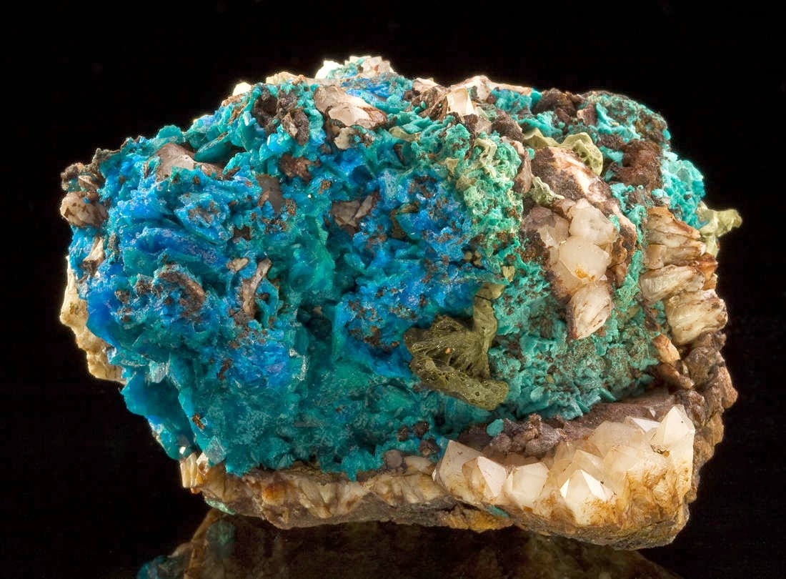
In order to understand the spread of marine life, Dr. Nakamura studies benthos, which are animals that are sessile or hardly move in the adult stage. They include deep-sea limpets, reef-building corals, and coral predator crown-of-thorns starfish. In autumn 2011, she boarded a deep-sea research vessel of the Japan Agency for Marine-Earth Science and Technology (JAMSTEC) to collect samples of deep-sea benthos from hydrothermal vents in the Okinawa Trough. Hydrothermal vents, where heated, mineral-laden seawater spews from cracks in the ocean crust, are home to various diverse organisms. From the collected samples, Nakamura took some deep-sea limpets back to her laboratory to study their population formation and colonization patterns. She did this by examining two characteristics: shell length and distribution pattern. Each sample was carefully measured to examine the time the sample has lived in a colony. The longer the shell length, the longer the inhabitance.

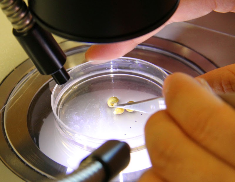
To understand the distribution patterns, Nakamura studies the fertilization process of limpets. Through microscopic observation of tissue sections from limpet gonads, she confirmed the stages of egg and sperm development. While limpets have distinct male and female sexes, the female has a bag-like organ called a spermatheca to store sperms for internal fertilization. Nakamura also discovered that eggs and sperms in various stages of maturity coexist simultaneously within the limpet’s genital glands. The limpets undergo a continual fertilization process in which each egg is spawned when it reaches maturity. This is different from coral fertilization, in which numerous mature eggs and sperms are released simultaneously and fertilized in the water. Fertilized limpet eggs released into the sea drift through the larval stage of growth, eventually finding home and adhering to the seabed to join a benthos community. The OIST Marine Biophysics Unit to which Dr. Nakamura belongs also studies ocean currents, which have considerable impact on the spread of benthic larvae. The team is trying to understand life history traits of benthos at the initial stage and the influence of ocean currents in order to find out how these organisms expand their habitat and respond to environmental changes.

Dr. Nakamura goes out on the water and observes marine organisms first hand. This approach is rooted in her belief that certain things can only be understood through observation of their natural state, and that the information obtained through these observations should be valued. “I would like to pass along to the next generation of researchers a diligent field research approach to understand ecosystems,” Dr. Nakamura said. By accumulating the understanding of the ecology of small marine organisms, she hopes to deepen an understanding of the spread of life in the entire ocean.

Note : The above story is based on materials provided by Okinawa Institute of Science and Technology – OIST.

Manganite

May 29, 2014

Table of Contents

Chemical Formula: MnO(OH)
Locality: Ilfeld, Harz, Germany
Name Origin: Named after its chemical composition.

Manganite is a mineral. Its composition is manganese oxide-hydroxide, MnO(OH), crystallizing in the monoclinic system (pseudo-orthorhombic). Crystals of manganite are prismatic and deeply striated parallel to their length; they are often grouped together in bundles. The color is dark steel-grey to iron-black, and the luster brilliant and submetallic. The streak is dark reddish-brown. The hardness is 4, and the specific gravity is 4.3. There is a perfect cleavage parallel to the brachypinacoid, and less-perfect cleavage parallel to the prism faces. Twinned crystals are not infrequent.

The mineral contains 89.7% manganese sesquioxide; it dissolves in hydrochloric acid with evolution of chlorine.

Occurrence

Manganite occurs with other manganese oxides in deposits formed by circulating meteoric water in the weathering environment in clay deposits and laterites. It forms by low temperature hydrothermal action in veins in association with calcite, barite, and siderite. Often associated with pyrolusite, braunite, hausmannite and goethite.

Manganite occurs in specimens exhibiting good crystal form at Ilfeld in the Harz Mountains of Germany, where the mineral occurs with calcite and barite in veins traversing porphyry. Crystals have also been found at Ilmenau in Thuringia, Neukirch near Sélestat in Alsace (newkirkite), Granam near Towie in Aberdeenshire, and in Upton Pyne near Exeter, UK and Negaunee, Michigan, United States, and in the Pilbarra of Western Australia. Good crystals have also been found at Atikokan, Ontario and Nova Scotia, Canada. As an ore of manganese it is much less abundant than pyrolusite or psilomelane.

Although described with various other names as early as 1772, the name manganite was first applied in a publication by W. Haidinger in 1827.

History

Discovery date : 1827
Town of Origin : ILFELD,HARZ
Country of Origin: ALLEMAGNE

Optical properties

Optical and misc. Properties : Opaque
Reflective Power : ~17%

Physical Properties

Cleavage: {010} Perfect
Color: Black, Gray, Grayish black.
Density: 4.3 – 4.4, Average = 4.34
Diaphaneity: Opaque
Fracture: Brittle – Generally displayed by glasses and most non-metallic minerals.
Hardness: 4 – Fluorite
Luminescence: Non-fluorescent.
Luster: Sub Metallic
Magnetism: Nonmagnetic
Streak: dark brown

Photos:

Manganite Ilfeld, Harz Mountains, Germany Miniature, 4.8 x 1.3 x 1 cm © irocks

Manganite 8.0×5.0x2.8 cm Caland Ore Properties Atikokan Ontario, Canada Copyright © David K. Joyce Minerals

Manganite Ilfeld, Nordhausen, Harz Mts, Thuringia, Germany Size: 4.0 x 3.0 x 1.5 cm (miniature) © danweinrich

N’Chwaning II Mine, N’Chwaning Mines, Kuruman, Kalahari manganese field, Northern Cape Province, South Africa

Four-billion-year-old rocks yield clues about Earth’s earliest crust

May 29, 2014

A sample of ancient rock from the Acasta Gneiss Complex in the Northwest Territories. Credit: Image courtesy of University of Alberta

It looks like just another rock, but what Jesse Reimink holds in his hands is a four-billion-year-old chunk of an ancient protocontinent that holds clues about how Earth’s first continents formed.
The University of Alberta geochemistry student spent the better part of three years collecting and studying ancient rock samples from the Acasta Gneiss Complex in the Northwest Territories, part of his PhD research to understand the environment in which they formed.

“The timing and mode of continental crust formation throughout Earth’s history is a controversial topic in early Earth sciences,” says Reimink, lead author of a new study in Nature Geoscience that points to Iceland as a solid comparison for how the earliest continents formed.

Continents today form when one tectonic plate shifts beneath another into Earth’s mantle and cause magma to rise to the surface, a process called subduction. It’s unclear whether plate tectonics existed 2.5 billion to four billion years ago or if another process was at play, says Reimink.

One theory is the first continents formed in the ocean as liquid magma rose from Earth’s mantle before cooling and solidifying into a crust.

Iceland’s crust formed when magma from the mantle rises to shallow levels, incorporating previously formed volcanic rocks. For this reason, Reimink says Iceland is considered a theoretical analogue on early Earth continental crust formation.

Ancient rocks 3.6 to four billion years old

A sample of ancient rock from the Acasta Gneiss Complex in the Northwest Territories

Working under the supervision of co-author Tom Chacko, Reimink spent his summers in the field collecting rock samples from the Acasta Gneiss Complex, which was discovered in the 1980s and found to contain some of Earth’s oldest rocks, between 3.6 and four billion years old. Due to their extreme age, the rocks have undergone multiple metamorphic events, making it difficult to understand their geochemistry, Reimink says.

Fortunately, a few rocks — which the research team dubbed “Idiwhaa” meaning “ancient” in the local Tlicho dialect — were better preserved. This provided a “window” to see the samples’ geochemical characteristics, which Reimink says showed crust-forming processes that are very similar to those occurring in present-day Iceland.

“This provides the first physical evidence that a setting similar to modern Iceland was present on the early Earth.”

These ancient rocks are among the oldest samples of protocontinental crust that we have, he adds, and may have helped jump-start the formation of the rest of the continental crust.

Reimink, who came to the U of A to work with Chacko, says the university’s lab resources are “second to none,” particularly the Ion Microprobe facility within the Canadian Centre for Isotopic Microanalysis run by co-author Richard Stern, which was instrumental to the discovery.

“That lab is producing some of the best data of its kind in the world. That was very key to this project.”

Note : The above story is based on materials provided by University of Alberta.

NASA missions let scientists see moon’s dancing tide from orbit

May 29, 2014

Illustration of Earth as seen from the moon. The gravitational tug-of-war between Earth and the moon raises a small bulge on the moon. The position of this bulge shifts slightly over time. Credit: NASA’s Goddard Space Flight Center

Scientists combined observations from two NASA missions to check out the moon’s lopsided shape and how it changes under Earth’s sway — a response not seen from orbit before.
The team drew on studies by NASA’s Lunar Reconnaissance Orbiter, which has been investigating the moon since 2009, and by NASA’s Gravity Recovery and Interior Laboratory, or GRAIL, mission. Because orbiting spacecraft gathered the data, the scientists were able to take the entire moon into account, not just the side that can be observed from Earth.

“The deformation of the moon due to Earth’s pull is very challenging to measure, but learning more about it gives us clues about the interior of the moon,” said Erwan Mazarico, a scientist with the Massachusetts Institute of Technology in Cambridge, Mass., who works at NASA’s Goddard Space Flight Center in Greenbelt, Md.

The lopsided shape of the moon is one result of its gravitational tug-of-war with Earth. The mutual pulling of the two bodies is powerful enough to stretch them both, so they wind up shaped a little like two eggs with their ends pointing toward one another. On Earth, the tension has an especially strong effect on the oceans, because water moves so freely, and is the driving force behind tides.

Earth’s distorting effect on the moon, called the lunar body tide, is more difficult to detect, because the moon is solid except for its small core. Even so, there is enough force to raise a bulge about 20 inches (51 centimeters) high on the near side of the moon and similar one on the far side.

The position of the bulge actually shifts a few inches over time. Although the same side of the moon constantly faces Earth, because of the tilt and shape of the moon’s orbit, the side facing Earth appears to wobble. From the moon’s viewpoint, Earth doesn’t sit motionless but moves around within a small patch of sky. The bulge responds to Earth’s movements like a dance partner, following wherever the lead goes.

“If nothing changed on the moon — if there were no lunar body tide or if its tide were completely static — then every time scientists measured the surface height at a particular location, they would get the same value,” said Mike Barker, a Sigma Space Corporation scientist based at Goddard and co-author of the new study, which is available online in Geophysical Research Letters.

A few studies of these subtle changes were conducted previously from Earth. But not until LRO and GRAIL did satellites provide enough resolution to see the lunar tide from orbit.

To search for the tide’s signature, the scientists turned to data taken by LRO’s Lunar Orbiter Laser Altimeter, or LOLA, which is mapping the height of features on the moon’s surface. The team chose spots that the spacecraft has passed over more than once, each time approaching along a different flight path. More than 350,000 locations were selected, covering areas on the near and far sides of the moon.

The researchers precisely matched measurements taken at the same spot and calculated whether the height had risen or fallen from one satellite pass to the next; a change indicated a shift in the location of the bulge.

A crucial step in the process was to pinpoint exactly how far above the surface LRO was located for each measurement. To reconstruct the spacecraft’s orbit with sufficient accuracy, the researchers needed the detailed map of the moon’s gravity field provided by the GRAIL mission.

“This study provides a more direct measurement of the lunar body tide and much more comprehensive coverage than has been achieved before,” said John Keller, LRO project scientist at Goddard.

The good news for lunar scientists is that the new results are consistent with earlier findings. The estimated size of the tide confirmed the previous measurement of the bulge. The other value of great interest to researchers is the overall stiffness of the moon, known as the Love number h2, and this was also similar to prior results.

Having confirmation of the previous values — with significantly smaller errors than before — will make the lunar body tide a more useful piece of information for scientists.

“This research shows the power of bringing together the capabilities of two missions. The extraction of the tide from the LOLA data would have been impossible without the gravity model of the moon provided by the GRAIL mission,” said David Smith, the principal investigator for LRO’s LOLA instrument and the deputy principal investigator for the GRAIL mission. Smith is affiliated with Goddard and the Massachusetts Institute of Technology.

Note : The above story is based on materials provided by NASA/Goddard Space Flight Center.

Magnetite

May 28, 2014

Table of Contents

Chemical Formula: Fe²⁺Fe³⁺₂O₄
Locality: Many localities and environments world wide.
Name Origin: Named for Magnes, a Geek shepherd, who discovered the mineral on Mt, Ida, He noted that the nails of his shoe and the iron ferrule of his staff clung to a rock.

Magnetite is a mineral, one of the three common naturally occurring iron oxides (chemical formula Fe₃O₄) and a member of the spinel group. Magnetite is the most magnetic of all the naturally occurring minerals on Earth. Naturally magnetized pieces of magnetite, called lodestone, will attract small pieces of iron, and this was how ancient people first noticed the property of magnetism.

Small grains of magnetite occur in almost all igneous and metamorphic rocks. Magnetite is black or brownish-black with a metallic luster, has a Mohs hardness of 5–6 and a black streak.

The chemical IUPAC name is iron(II,III) oxide and the common chemical name is ferrous-ferric oxide.

History

Discovery date : 1845
Town of Origin : MAGNESIA, THESSALIE
Country of Origin : GRECE

Optical properties

Optical and misc. Properties : Opaque
Reflective Power : ~21%

Physical Properties

Cleavage: None
Color: Grayish black, Iron black.
Density: 5.1 – 5.2, Average = 5.15
Diaphaneity: Opaque
Fracture: Sub Conchoidal – Fractures developed in brittle materials characterized by semi-curving surfaces.
Hardness: 5.5-6 – Knife Blade-Orthoclase
Luminescence: Non-fluorescent.
Luster: Metallic
Magnetism: Naturally strong
Streak: black

Photos :

Magnetite 5.6×5.6×3.8 cm Bentley Lake Faraday Mine Property Ontario, Canada Copyright © David K. Joyce Minerals

Magnetite ZCA Mine No. 4, Balmat, St Lawrence Co., New York, USA Cabinet, 11.9 x 11.0 x 9.5 cm © irocks

Magnetite ZCA Mine, Balmat, St Lawrence County, New York, USA Cabinet, 11.5 x 4.6 x 4.5 cm © irocks

Rio Varbore, Manubiola Valley, Berceto, Parma Province, Emilia-Romagna, Italy © Chinellato Matteo

High-resolution images shed light on dinosaur bone healing

May 28, 2014

Scientists have used a highly sensitive, high-resolution X-ray scanning technique to detect minute quantities of chemicals associated with bone healing in 150-million-year-old dinosaur bones.

They looked in cracks, fractures and breaks in the ancient remains, and found traces of copper, zinc and strontium, which are essential for enzymes involved with bone maintenance, repair and healing.
As well as shedding light on the differences between normal and healed bone, the findings give the first chemical clues to how the dinosaurs’ bones may have healed when they were injured.

They also suggest that many predatory dinosaurs may have recovered from the impact of massive trauma, which would likely kill you or me.

The findings are published in Journal of the Royal Society Interface.

‘It seems dinosaurs evolved a splendid suite of defence mechanisms to help regulate the healing and repair of injuries. Not a lot is known about the biochemistry of healing in extinct animals. So, the ability to diagnose such processes some 150 million years later might well shed light on how we can use Jurassic chemistry in the 21st century,’ says Dr Phil Manning of the University of Manchester, one of the study’s co-authors.

Fossilised bones sometimes show evidence of trauma, sickness and subsequent signs healing. Working out what happened to them usually relies on scientists slicing through ancient, valuable specimens to analyse them.

Manning and colleagues from UK and US universities realised that looking at so-called chemical signatures in the bones could uncover details about how they healed.

‘This is because the body uses a distinct suite of trace-metal co-ordinated enzymes to repair bones,’ explains Manning.

‘Copper-based enzymes are associated with forming calluses. The second stage of bone repair involves zinc-containing enzymes, which promotes bone growth. And the final stage to check all the work done is good involves an enzyme that contains strontium,’ he adds.

‘So if you’re imaging a healed fracture, you’ll find trace amounts of strontium evenly distributed along the healed bone. But if it’s still healing, there’ll be higher concentrations of zinc.’

These elements make up much less than one per cent of our entire bodies, which means trying to find them in 150-million-year-old fossils is a big ask.

The interdisciplinary team based at the University of Manchester used both the Stanford Synchrotron Radiation Light Source and Diamond Light Source to analyse a bone from a theropod dinosaur called Allosaurus fragilis.

The predatory Allosaurus, which means ‘different lizard’, lived 155 to 150 million years ago during the late Jurassic Period. It was a member of a group of vertebrates called the archosaurs, whose modern members include the crocodiles and birds.

The researchers also used the Stanford synchrotron to analyse a bone from a living archosaur, the turkey vulture.

‘Theropods are a logical study group as they are more closely related to the most diverse group of extant archosaurs, the birds,’ explain the authors.

Synchrotron particle accelerators act like a giant microscope, harnessing the power of electrons to produce light brighter than a billion suns to study anything from jet engines to viruses and vaccines.

The team used extremely bright light produced by the two particle accelerators to find minute traces of zinc, copper and strontium in the bones.

‘You can only detect such chemistry using a synchrotron, because this technique permits you to exactly image the relationship of each atom to its surrounding elements. This allows you to identify if the element was part of the bone-healing process, or if it came from the environment in which the bone became fossilised,’ says Manning.

When they compared the chemical signatures in the dinosaur and turkey vulture specimens, they expected them to be fairly similar.

But they found that the dinosaur bone revealed signs of fracture healing that are more reminiscent of that of modern reptiles like crocodiles or alligators.

‘It is quite possible you’ve got a reptilian-style repair mechanism combined with elevated metabolism, like that you’d find in alligators and birds respectively. So you’ve got a double whammy in a good way. If you suffer massive trauma, you’ve got the perfect set-up to survive it,’ says Manning.

‘Bones doesn’t form scar tissue, like a scratch to your skin, so the body has to completely reform new bone following the same stages that occurred at the skeleton grew in the first place. The means we are able to tease out the chemistry of bone development through such pathological studies,’ says Jennifer Anné, PhD student at the University of Manchester, first author of the study.

‘You’re basically seeing a biological process preserved in the sands of time,’ adds Manning.

More Information :
Jennifer Anné, Nicholas P. Edwards, Roy A. Wogelius, Allison R. Tumarkin-Deratzian, William I. Sellers, Arjen van Veelen, Uwe Bergmann, Dimosthensis Sokaras, Roberto Alonso-Mori, Konstantin Ignatyev, Victoria M. Egerton and Phillip L. Manning, Synchrotron imaging reveals bone healing and remodelling strategies in extinct and extant vertebrates, Journal of the Royal Society Interface, published 7th May 2014, http://dx.doi.org/10.1098/rsif.2014.0277

Note : The above story is based on materials provided by © Natural Environment Research Council

Antarctic Ice Sheet unstable at end of last ice age, new study finds

May 28, 2014

This is one of many icebergs that sheared off the continent and ended up in the Scotia Sea. Credit: Michael Weber, University of Cologne

A new study has found that the Antarctic Ice Sheet began melting about 5,000 years earlier than previously thought coming out of the last ice age – and that shrinkage of the vast ice sheet accelerated during eight distinct episodes, causing rapid sea level rise.
The international study, funded in part by the National Science Foundation, is particularly important coming on the heels of recent studies that suggest destabilization of part of the West Antarctic Ice Sheet has begun.

Results of this latest study are being published this week in the journal Nature. It was conducted by researchers at University of Cologne, Oregon State University, the Alfred-Wegener-Institute, University of Hawaii at Manoa, University of Lapland, University of New South Wales, and University of Bonn.

The researchers examined two sediment cores from the Scotia Sea between Antarctica and South America that contained “iceberg-rafted debris” that had been scraped off Antarctica by moving ice and deposited via icebergs into the sea. As the icebergs melted, they dropped the minerals into the seafloor sediments, giving scientists a glimpse at the past behavior of the Antarctic Ice Sheet.

Periods of rapid increases in iceberg-rafted debris suggest that more icebergs were being released by the Antarctic Ice Sheet. The researchers discovered increased amounts of debris during eight separate episodes beginning as early as 20,000 years ago, and continuing until 9,000 years ago.

The melting of the Antarctic Ice Sheet wasn’t thought to have started, however, until 14,000 years ago.

“Conventional thinking based on past research is that the Antarctic Ice Sheet has been relatively stable since the last ice age, that it began to melt relatively late during the deglaciation process, and that its decline was slow and steady until it reached its present size,” said lead author Michael Weber, a scientist from the University of Cologne in Germany.

“The sediment record suggests a different pattern – one that is more episodic and suggests that parts of the ice sheet repeatedly became unstable during the last deglaciation,” Weber added.

The research also provides the first solid evidence that the Antarctic Ice Sheet contributed to what is known as meltwater pulse 1A, a period of very rapid sea level rise that began some 14,500 years ago, according to Peter Clark, an Oregon State University paleoclimatologist and co-author on the study.

The largest of the eight episodic pulses outlined in the new Nature study coincides with meltwater pulse 1A.

“During that time, the sea level on a global basis rose about 50 feet in just 350 years – or about 20 times faster than sea level rise over the last century,” noted Clark, a professor in Oregon State’s College of Earth, Ocean, and Atmospheric Sciences. “We don’t yet know what triggered these eight episodes or pulses, but it appears that once the melting of the ice sheet began it was amplified by physical processes.”

The researchers suspect that a feedback mechanism may have accelerated the melting, possibly by changing ocean circulation that brought warmer water to the Antarctic subsurface, according to co-author Axel Timmermann, a climate researcher at the University of Hawaii at Manoa.

“This positive feedback is a perfect recipe for rapid sea level rise,” Timmermann said.

Some 9,000 years ago, the episodic pulses of melting stopped, the researchers say.

“Just as we are unsure of what triggered these eight pulses,” Clark said, “we don’t know why they stopped. Perhaps the sheet ran out of ice that was vulnerable to the physical changes that were taking place. However, our new results suggest that the Antarctic Ice Sheet is more unstable than previously considered.”

Today, the annual calving of icebergs from Antarctic represents more than half of the annual loss of mass of the Antarctic Ice Sheet – an estimated 1,300 to 2,000 gigatons (a gigaton is a billion tons). Some of these giant icebergs are longer than 18 kilometers.

More information: Paper: Millennial-scale variability in Antarctic ice-sheet discharge during the last deglaciation, dx.doi.org/10.1038/nature13397

Note : The above story is based on materials provided by Oregon State University

Magnesite

May 28, 2014

Table of Contents

Chemical Formula: MgCO₃
Locality: Magnisía (Magnesia) Prefecture, Thessalia (Thessaly) Department, Greece
Name Origin: Named after its chemical composition.

Magnesite is a mineral with the chemical formula MgCO₃ (magnesium carbonate). Mixed crystals of iron II carbonate and magnesite (mixed crystals known as ankerite) possess a layered structure: monolayers of carbonate groups alternate with magnesium monolayers as well as iron II carbonate monolayers. Manganese, cobalt and nickel may also occur in small amounts.

Occurrence

Magnesite occurs as veins in and an alteration product of ultramafic rocks, serpentinite and other magnesium rich rock types in both contact and regional metamorphic terrains. These magnesites often are cryptocrystalline and contain silica in the form of opal or chert.

Magnesite is also present within the regolith above ultramafic rocks as a secondary carbonate within soil and subsoil, where it is deposited as a consequence of dissolution of magnesium-bearing minerals by carbon dioxide within groundwaters.

History

Discovery date : 1808
Town of Origin : MAGNESIA, THESSALIE
Country of Origin : GRECE

Optical properties

Optical and misc. Properties : Transparent to translucent to opaque
Refractive Index : from 1,50 to 1,70

Physical Properties

Cleavage: {1011} Perfect, {1011} Perfect, {1011} Perfect
Color: Colorless, White, Grayish white, Yellowish white, Brownish white.
Density: 3
Diaphaneity: Transparent to translucent to opaque
Fracture: Brittle – Conchoidal – Very brittle fracture producing small, conchoidal fragments.
Hardness: 4 – Fluorite
Luminescence: Fluorescent, Short UV=blue white, Long UV=bright blue white.
Luster: Vitreous (Glassy)
Streak: white

Photos :

Uvite with Magnesite Brumado, Bahia, Brazil Size: 7.0 x 6.0 x 6.0 cm (small cabinet) © danweinrich

Uvite with Magnesite Brumado, Bahia, Brazil Size: 2.5 x 2.0 x 1.3 cm (thumbnail) © danweinrich

Magnesite Bahia, Brazil Thumbnail, 12.7 x 8.0 mm ; 3.52 carats © irocks

Beryl var. Emerald with Magnesite Brumado, Bahia, Brazil Size: 6.3 x 2.0 x 1.8 cm (miniature) © danweinrich

Pomba pit, Serra das Éguas, Brumado (Bom Jesus dos Meiras), Bahia, Brazil © Rob Lavinsky

Where have all the craters gone?

May 28, 2014

Impact craters reveal one of the most spectacular geologic process known to man. During the past 3.5 billion years, it is estimated that more than 80 bodies, larger than the dinosaur-killing asteroid that struck the Yucatan Peninsula 66 million years ago, have bombarded Earth. However, tectonic processes, weathering, and burial quickly obscure or destroy craters. For example, if Earth weren’t so dynamic, its surface would be heavily cratered like the Moon or Mercury.

Work by B.C. Johnson and T.J. Bowling predicts that only about four of the craters produced by these impacts could persist until today, and geologists have already found three such craters (larger than 170 km in diameter). Their study, published online for Geology on 22 May 2014, indicates that craters on Earth cannot be used to understand Earth’s bombardment history.

Johnson and Bowling write, however, that layers of molten rock blasted out early in the impact process may act as better records of impacts—even after the active Earth has destroyed the source craters. The authors suggest that searches for these impact ejecta layers will be more fruitful for determining how many times Earth was hit by big asteroids than searches for large craters.

Reference:
B.C. Johnson and T.J. Bowling. Where have all the craters gone? “Earth’s bombardment history and the expected terrestrial cratering record.” Geology, G35754.1, first published on May 22, 2014, DOI: 10.1130/G35754.1

Note : The above story is based on materials provided by Geological Society of America

Slave River

May 28, 2014

Table of Contents

The Slave River is a Canadian river that flows from Lake Athabasca in northeastern Alberta and empties into Great Slave Lake in the Northwest Territories. The river’s name is thought to derive from the name for the Slavey group of the Dene First Nations, Deh Gah Got’ine, in the Athabaskan language, and has nothing to do with slavery. The Chipewyan had displaced other native people from this region.

Course

The Slave River originates in the Peace-Athabasca Delta, at the forks of Peace River and Riviere Des Roches, which drains the Athabasca River and Lake Athabasca. The Slave River flows north into the Northwest Territories and into the Great Slave Lake north of Fort Resolution. From there the water reaches the Arctic Ocean through the Mackenzie River.The river is 434 km in length and has a cumulative drainage area of 616,400 km².

Portage and Navigation

Prior to the extension of railway service to Hay River, Northwest Territories, a river port on Great Slave Lake, cargo shipment on the Slave River was an important transport route. Locally built wooden vessels were navigating the river into the late 19th Century. The rapids required a portage of 16 miles (26 km). Tractors were imported from Germany to assist in hauling goods around the rapids. Tugs and barges of the Northern Transportation Company’s “Radium Line” were constructed in the south and disassembled. The parts were then shipped by rail to Waterways, Alberta, shipped by barge to the portage, and portaged to the lower river for reassembly, where they could navigate most of the rest of the extensive Mackenzie River basin.

Tributaries

Peace-Athabasca Delta
- Athabasca River
- Lake Athabasca
- Riviere Des Roches
- Chilloneys Creek
- Revillon Coupe
- Dempsey Creek
- Peace River
- Scow Channel
- Murdock Creek
- Darough Creek

Powder Creek
La Butte Creek
Hornaday River
Salt River
Little Buffalo River

Note : The above story is based on materials provided by Wikipedia

Ludlockite

May 27, 2014

Table of Contents

Chemical Formula: PbFe³⁺₄As³⁺₁₀O₂₂
Locality: In a boulder of ore found at Tsumeb, Namibia.
Name Origin: Named for mineral dealers Ludlow Smith and Locke Key, who discovered the mineral.

History

Discovery date : 1970
Town of Origin : TSUMEB
Country of Origin : NAMIBIE

Optical properties

Refractive Index: from 1,96 to 2,12

Physical Properties

Cleavage: {011} Perfect, {021} Perfect
Color: Reddish brown.
Density: 4.37 – 4.4, Average = 4.38
Hardness: 1.5-2 – Talc-Gypsum
Luster: Subadamantine
Streak: pale brown

Photos :

Ludlockite, Philipsbornite $85.00 2.1×1.7×1.7 cm Tsumeb Namibia Copyright © David K. Joyce Minerals

Ludlockite with Leiteite and yellow unknown Tsumeb Mine, Tsumeb, Otjikoto Region, Namibia Size: 4.0 x 3.0 x 2.0 cm (miniature) © danweinrich

Ludlockite Tsumeb Mine, Tsumeb, Otjikoto Region, Namibia Miniature, 3.9 x 2.3 x 1.5 cm © irocks

Tsumeb Mine (Tsumcorp Mine), Tsumeb, Otjikoto Region (Oshikoto), Namibia © Paul De Bondt

Seafloor experts publish new view of zone where Malaysia Airlines flight 370 might lie

May 27, 2014

Seafloor topography in the Malaysia Airlines flight MH370 search area. Dashed lines approximate the search zone for sonar pings emitted by the flight data recorder and cockpit voice recorder popularly called black boxes. The first sonar contact (black circle) was reportedly made by a Chinese vessel on the east flank of Batavia Plateau (B), where the shallowest point in the area (S) is at an estimated depth of 1637 meters. The next reported sonar contact (red circle) was made by an Australian vessel on the north flank of Zenith Plateau (Z). The deepest point in the area (D) lies in the Wallaby-Zenith Fracture Zone at an estimated depth of 7883 meters. The Wallaby Plateau (W) lies to the east of the Zenith Plateau. The shallowest point in the entire area shown here is on Broken Ridge (BR). Deep Sea Drilling Project (DSDP) site 256 is marked by a gray dot. The inset in the top left shows the area’s location to the west of Australia. Seafloor depths are from the General Bathymetric Chart of the Oceans [2010]. Credit: Walter H.F. Smith and Karen M. Marks

A new illustration of the seafloor, created by two of the world’s leading ocean floor mapping experts that details underwater terrain where the missing Malaysia Airlines flight might be located, could shed additional light on what type of underwater vehicles might be used to find the missing airplane and where any debris from the crash might lie.
The seafloor topography map illustrates jagged plateaus, ridges and other underwater features of a large area underneath the Indian Ocean where search efforts have focused since contact with Malaysia Airlines flight MH370 was lost on March 8. The image was published today in Eos, the weekly newspaper of the Earth and space sciences, published by the American Geophysical Union.

The new illustration of a 2,000 kilometer by 1,400 kilometer (1,243 miles by 870 miles) area where the plane might be shows locations on the seafloor corresponding to where acoustic signals from the airplane’s black boxes were reportedly detected at the surface by two vessels in the area. It also shows the two plateaus near where these “pings” were heard.

It points out the deepest point in the area: 7,883 meters (about five miles) underneath the sea in the Wallaby-Zenith Fracture Zone — about as deep as 20 Empire State buildings stacked top to bottom. Undersea mountains and plateaus rise nearly 5,000 meters (about three miles) above the deep seafloor, according to the map.

The illustration, designated as Figure 1 of the Eos article, was created by Walter H.F. Smith and Karen M. Marks, both of the National Oceanic and Atmospheric Administration’s Laboratory for Satellite Altimetry in College Park, Maryland, and the former and current chairs, respectively, of the Technical Sub-Committee on Ocean Mapping of the General Bathymetric Chart of the Oceans, or GEBCO. GEBCO is an international organization that aims to provide the most authoritative publicly available maps of the depths and shapes of the terrain underneath the world’s oceans.

Satellite altimetry has made it possible to depict the topography of vast regions of the seafloor that would otherwise have remained unmapped, Smith said. To illustrate the topography of the search area, Smith and Marks used publicly available data from GEBCO and other bathymetric models and data banks, along with information culled from news reports.

Smith said the terrain and depths shown in the map could help searchers choose the appropriate underwater robotic vehicles they might use to look for the missing plane. Knowing the roughness and shape of the ocean floor could also help inform models predicting where floating debris from the airplane might turn up.

Smith cautions that the new illustration is not a roadmap to find the missing airplane. Nor does the map define the official search area for the aircraft, he added.

“It is not ‘x marks the spot’,” Smith said of their map. “We are painting with a very, very broad brush.”

Search efforts for the missing airplane have focused on an area of the southern Indian Ocean west of Australia where officials suspect that the plane crashed after it veered off course. After an initial air and underwater search failed to find any trace of the airplane, authorities announced this month that they will expand the search area and also map the seabed in the area.

Smith pointed out that the search for the missing plane is made more difficult because so little is understood about the seafloor in this part of the Indian Ocean. In the southeast Indian Ocean, only 5 percent of the ocean bottom has been measured by ships with echo soundings. Knowledge of the rest of the area comes from satellite altimetry, which provides relatively low-resolution mapping compared to ship-borne methods.

“It is a very complex part of the world that is very poorly known,” Smith said.

A lack of good data about Earth’s seafloors not only hinders search efforts, it also makes it harder for scientists to accurately model the world’s environment and climate, Smith noted. Today, our knowledge of our planet’s undersea topography is “vastly poorer than our knowledge of the topographies of Earth’s Moon, Mars and Venus,” Smith and Marks write in Eos. This is because these other planetary bodies have no oceans, making their surfaces relatively easy to sense from space.

Smith said he hoped that “the data collected during the search for MH370 will be contributed to public data banks and will be a start of greater efforts to map Earth’s ocean floor.”

Note : The above story is based on materials provided by American Geophysical Union.

Research suggests more silicon in Earth’s lower mantle than thought

May 27, 2014

For many years geophysicists have argued over the perplexing mystery regarding the amount of silicon in the Earth’s mantle that is thought to have arrived there via impacts with asteroids.
The problem is that tests done to determine the composition of the mantel have found that there appears to be less silicon in it proportionally, than there is in asteroids. Now new research by a Japanese team suggests that the lowest section of the Earth’s mantle has more silicon in it than does the upper parts, perhaps solving the mystery. They have described their work in their paper published in the journal Nature.

To help clarify what lies far beneath our feet, geophysicists have subdivided the Earth’s mantle into three broad sections: the upper, middle and lower mantle. The upper mantle describes the crust and approximately 400 km below. The middle is about 250 km thick and the lower goes to about 2,900 km in depth.

The upper mantle is far easier to study of course, due to its proximity and thus the proportion of silicon in it is well understood. Not so well understood has been the composition of the middle and lower mantles. To study them, researches generally use seismic data recorded by sending shockwaves into the ground, but doing so thus far, has led more often to speculation than good science.

To get a better handle on what is happening so far beneath the Earth’s surface the Japanese team took a different approach; instead of trying to measure the lower mantle itself, they sought to recreate it in a lab where it could be measured much more easily. To do that, they mixed the ingredients (mainly silicate perovskite and ferropericlase) they believe exist in the lower mantel and placed them in a pressure chamber. There the sample was subjected to different pressure levels consistent with current theories describing the differing degrees of pressure at different levels of the mantle. They then applied the same seismic tests normally done on the real mantle. In so doing, they have come to believe that the lower mantle has a volume that is approximately 93% silicate perovskite, which when compared with data describing the upper crust gives an average amount of silicon for the entire mantle that is very nearly equal to that found in asteroids. Thus, the mystery, they say is solved.

More information: Nature 485, 90–94 (03 May 2012) doi:10.1038/nature11004

Ludlamite

May 27, 2014

Table of Contents

Chemical Formula: (Fe,Mn,Mg)₃(PO₄)₂·4H₂O
Locality: Wheal Jane, Kea, near Truro, Cornwall, England, UK.
Name Origin: Named for Henry Ludlam (1824-1880), English mineralogist and collector.

Ludlamite is a rare phosphate mineral with formula: (Fe,Mn,Mg)₃(PO₄)₂·4H₂O

It was first described in 1877 for an occurrence in Wheal Jane mine in Cornwall, England and named for English mineralogist Henry Ludlam (1824–1880).

History

Discovery date : 1877
Town of Origin : WHEAL JANE (MINE), TRURO, CORNOUAILLES
Country of Origin: ANGLETERRE

Optical properties

Optical and misc. Properties : Transparent to Translucent
Refractive Index: from 1,65 to 1,69
Axial angle 2V : 82°

Physical Properties

Cleavage: {001} Perfect, {100} Indistinct
Color: Apple green, Colorless, Green, Greenish white, Light green.
Density: 3.15
Diaphaneity: Transparent to Translucent
Hardness: 3.5 – Copper Penny
Luster: Vitreous (Glassy)
Streak: white

Photos :

Ludlamite Blackbird Mine, Lemhi Co., Idaho, USA Size: 2.8 x 2.5 x 0.6 cm (thumbnail) © danweinrich

Ludlamite Stari Trg Mine, Trepča complex, Trepča valley, Kosovska Mitrovica, Kosovo Specimen weight:25 gr. Crystal size:Up to 3 mm Overall size: 35mm x 27 mm x 25 mm © minservice

Ludlamite Huanuni Mine, Huanuni, Dalence Province, Oruro Department, Bolivia Size: 3.0 x 2.0 x 1.5 cm (thumbnail) © danweinrich

San Antonio Mine (San Antonio el Grande Mine), East Camp, Santa Eulalia District, Mun. de Aquiles Serdán, Chihuahua, Mexico © fabreminerals

Extreme-pressure research explores how Earth’s mantle solidified

May 27, 2014

During the earliest stages of the Earth’s formation, the planet’s mantle may have taken the form of a giant magma ocean, being fully or partially molten all the way down to the core-mantle boundary. Though today mantle material is predominantly solid, some scientists suggest that regions of anomalously low seismic wave velocity deep within the mantle, known as ultralow velocity zones (ULVZs), may be indicative of a remnant magma ocean or of partial melting of minerals near the core-mantle boundary. To understand how the early mantle solidified, or whether modern melt could be the source of ULVZs, scientists need to know how various minerals and melts behave under the extreme conditions found near the center of the Earth.

Through the use of various techniques, Thomas et al.analyzed how the density of molten fayalite—an iron-bearing silicate mineral—behaved under pressures up to 161 gigapascals, surpassing those at the core-mantle boundary.

The research adds to previous investigations into the equation of state of fayalite, an expression describing how the material’s density responds to changes in temperature and pressure. The authors find that iron-bearing fayalite behaves similarly to nonferrous silicate liquids during compression and heating.

Based on the measured equation of state, and on the known behavior of other silicate liquids, the authors suggest that the solidification of the Earth’s early mantle would have started near the core-mantle boundary or in the lower mantle.

Based on the current research, the authors are unable to determine whether ultralow velocity zones are necessarily caused by partial melting of the mantle material. They did, however, identify a potential set of liquid compositions that would be gravitationally stable if present.

Reference:
Journal of Geophysical Research – Solid Earth, doi:10.1029/2012JB009403, 2012

Note : The above story is based on materials provided by American Geophysical Union

Chronology of Christmas Island’s volcanic history unearthed

May 27, 2014

Researchers established the age of the various rocks on Christmas Island at the time they were erupted, and established the position of the island through time. Credit: Peter McKiernan

Geological samples from Christmas Island have been analysed by a West Australian scientist, giving valuable insight into its unique volcanic history.

Curtin University geochronologist Dr Fred Jourdan says while continents are often the subject of geological investigation, ocean geology is less studied and the results of the Christmas Island study adds important information to the field.

The report he co-authored has been published in Gondwana Research.

It describes the Christmas Island area as an extensive zone of volcanism in the north-east Indian Ocean, consisting of numerous submerged seamounts and flat topped guyots.

It explains the island has experienced multiple episodes of volcanism that are exposed sporadically along its coastline.

It is the only island in the region to show intraplate volcanism in the form of basaltic rocks that are exposed above sea level.

Dr Jourdan says the project was a collaboration with Macquarie University. Samples were collected by a student from Macquarie University and tested at Curtin University using 40Ar/39Ar geochronology and paleomagnetism.

Dr Jourdan says this is where the ‘real science’ of finding their origin began.

“What we did was two things; we established the age of the various rocks on the island at the time they were erupted, and we established the position of the island through time,” he says.

“We needed to look at where it was before, to understand why there is volcanic activity at all—is it random or related to something in particular?

“We measured two different ages but we know, comparing it to other seamounts, there are in fact three periods of volcanic activity.

Three stages of Christmas Island volcanic activity

“The oldest happened when Australia and India separated and the rock left behind melted to create a seamount—that was the first volcanic activity, although we didn’t sample this and at this time, the island was much further south than it is now.

“The second, happened between 43 and 37 million years ago—it happened when the continent moved north above a hot zone in the mantle.

“Nothing happened for 30 million years until, in its northward movement toward the European-Asian plate; the plate cracked five million years ago and the magma could easily rise through the cracks.”

Dr Jourdan says similar low volume intraplate volcanism had previously been observed at similar tectonic settings to the Japan and Tonga trench.

“…We put forward the Indo Australian plate subduction setting as a likely candidate for this phase of introceanic volcanism.”

More information:
Rajat Taneja, Craig O’Neill, Mark Lackie, Tracy Rushmer, Phil Schmidt, Fred Jourdan, “40Ar/39Ar geochronology and the paleoposition of Christmas Island (Australia), Northeast Indian Ocean,” Gondwana Research, Available online 27 April 2014, ISSN 1342-937X, dx.doi.org/10.1016/j.gr.2014.04.004.

Note : The above story is based on materials provided by Science Network WA

Löllingite “Loellingite”

May 26, 2014

Löllingite with Fluorite and Arsenopyrite Huanggang Mines, Kèshíkèténg Qí, Chifeng, Inner Mongolia A.R. China (2012) Specimen size: 7.5 × 6.5 × 6.2 cm = 3.0” × 2.6” × 2.4” Main crystal size: 5.8 × 5.7 cm = 2.3” × 2.2” © Fabre Minerals

Table of Contents

Chemical Formula: FeAs₂
Locality: Lölling, Hüttenberg, Carinthia, Austria
Name Origin: Named after its locality.

Loellingite, also spelled löllingite, is an iron arsenide mineral with formula FeAs₂. It is often found associated with arsenopyrite (FeAsS) from which it is hard to distinguish. Cobalt, nickel and sulfur substitute in the structure. The orthorhombic lollingite group includes the nickel iron arsenide rammelsbergite and the cobalt iron arsenide safflorite. Leucopyrite is an old synonym for loellingite.

It forms opaque silvery white orthorhombic prismatic crystals often exhibiting crystal twinning. It also occurs in anhedral masses and tarnishes on exposure to air. It has a Mohs hardness of 5.5 to 6 and a quite high specific gravity of 7.1 to 7.5. It becomes magnetic after heating.

Loellingite was first described in 1845 at the Lölling district in Carinthia, Austria, for which it was named.

It occurs in mesothermal ore deposits associated with skutterudite, native bismuth, nickeline, nickel-skutterudite, siderite and calcite. It has also been reported from pegmatites.

History

Discovery date : 1845
Town of Origin : MINE WOLFBAUER, LOLLING, HUTTENBERG, CARINTHIE
Country of Origin: AUTRICHE

Optical properties

Optical and misc. Properties: Opaque
Reflective Power: 51,7-54,2% (580)

Physical Properties

Cleavage: {001} Distinct
Color: Silvery white, Tarnish gray.
Density: 7.1 – 7.7, Average = 7.4
Diaphaneity: Opaque
Fracture: Uneven – Flat surfaces (not cleavage) fractured in an uneven pattern.
Hardness: 5 – Apatite
Luminescence: Non-fluorescent.
Luster: Metallic
Magnetism: Magnetic after heating
Streak: grayish black

Photos :

Arsenic crystals with Loellingite St. Andreasberg, Harz Mountains, Germany Miniature, 4.7 x 3.1 x 3.0 cm © irocks

Löllingite Crovino mine, Susa valley, Piedmont, Italy Specimen weight:30 gr. Crystal size:2 mm Overall size: 50mm x 32 mm x 28 mm © minservice

Löllingite Huanggang nr. 1 mine – Chifeng – Inner Mongolia – China Specimen weight:314 gr. Crystal size:mm. 24 Overall size: 72mm x 55 mm x 35 mm © minservice

Carlés Mine, Carlés, Salas, Asturias, Spain © JRGL

Earth’s magnetic field is important for climate change at high altitudes

May 26, 2014

New research, published this week, has provided scientists with greater insight into the climatic changes happening in the upper atmosphere. Scientists found that changes in the Earth’s magnetic field are more relevant for climatic changes in the upper atmosphere (about 100-500 km above the surface) than previously thought. Understanding the cause of long-term change in this area helps scientists to predict what will happen in the future. This has key implications for life back on earth.

A good understanding of the long-term behaviour of the upper atmosphere is essential; it affects a lot of satellite-based technology, such as global navigation systems and high-frequency radio communication systems. Some satellites even operate within the upper atmosphere itself.

The increase in atmospheric CO2 concentration has been thought to be the main cause of climatic changes at these high altitudes. This study suggests that magnetic field changes that have taken place over the past century are as important.

Both increasing levels of CO2 and changes in the Earth’s magnetic field affect the upper atmosphere, including its charged portion, also known as the ionosphere. Dr. Ingrid Cnossen from the British Antarctic Survey used computer simulations to compare the effects of these two factors over the past century.

While CO2 causes heat to be trapped in the lower atmosphere, it actually cools the upper atmosphere. The simulations show that the increase in CO2 concentration over the past 100 years has caused the upper atmosphere, at around 300 km altitude, to cool by around 8 degrees. At the same altitude, changes in the Earth’s magnetic field caused a similar amount of cooling over parts of North America, but caused a warming over other parts of the world, with the strongest warming, of up to 12 degrees, located over Antarctica.

Dr. Ingrid Cnossen said: “Computer simulations are a very important tool in understanding the causes of climate change at high altitudes. We still can’t explain all of the long-term trends that have been observed, but it helps that we now know how important the magnetic field is.”

The new simulations also indicate that rising CO2 levels have caused the densest part of the ionosphere to lower by about 5 km globally. Changes in the Earth’s magnetic field can cause much larger changes, but they are very dependent on location and can be either positive or negative; over the southern Atlantic Ocean a decrease in height of up to 50 km was found, while an increase in height of up to 20 km was found over western Africa.

The findings are published in the Journal of Space Weather and Space Climate.

Note : The above story is based on materials provided by British Antarctic Survey

Against the current with lava flows

May 26, 2014

A pit chain marks a subterranean lava tunnel. Its roof collapsed partially. Credit: Image: Mars Image Explorer / asu.edu

Table of Contents

Lava formed massive canyons on Mars

An Italian astronomer in the 19th century first described them as ‘canali’ – on Mars’ equatorial region, a conspicuous net-like system of deep gorges known as the Noctis Labyrinthus is clearly visible. The gorge system, in turn, leads into another massive canyon, the Valles Marineris, which is 4,000 km long, 200 km wide and 7 km deep. Both of these together would span the US completely from east to west.
As these gorges, when observed from orbit, resemble terrestrial canyons formed by water, most researchers assumed that immense flows of water must have carved the Noctis Labyrinthus and the Valles Marineris into the surface of Mars. Another possibility was that tectonic activity had created the largest rift valley on a planet in our solar system.

Lava flows caused the gorges

These assumptions were far from the mark, says Giovanni Leone, a specialist in planetary volcanism in the research group of ETH professor Paul Tackley. Only lava flows would have had the force and mass required to carve these gigantic gorges into the surface of Mars. The study was recently published in the Journal of Volcanology and Geothermal Research.

In recent years, Leone has examined intensively the structure of these canyons and their outlets into the Ares Vallis and the Chryse Planitia, a massive plain on Mars’ low northern latitude. He examined thousands of high-resolution surface images taken by numerous Mars probes, including the latest from the Mars Reconnaissance Orbiter, and which are available on the image databases of the US Geological Survey.

No discernible evidence of erosion by water

His conclusion is unequivocal: “Everything that I observed on those images were structures of lava flows as we know them on Earth,” he emphasises. “The typical indicators of erosion by water were not visible on any of them.” Leone therefore does not completely rules out water as final formative force. Evidence of water, such as salt deposits in locations where water evaporated from the ground or signs of erosion on the alluvial fans of the landslides, are scarce but still existing. “One must therefore ask oneself seriously how Valles Marineris could have been created by water if one can not find any massive and widespread evidence of it.” The Italian volcanologist similarly could find no explanation as to where the massive amounts of water that would be required to form such canyons might have originated.

Source region of lava flows identified

The explanatory model presented by Leone in his study illustrates the formation history from the source to the outlet of the gorge system. He identifies the volcanic region of Tharsis as the source region of the lava flows and from there initial lava tubes stretched to the edge of the Noctis Labyrinthus. When the pressure from an eruption subsided, some of the tube ceilings collapsed, leading to the formation of a chain of almost circular holes, the ‘pit chains’.

When lava flowed again through the tubes, the ceilings collapsed entirely, forming deep V-shaped troughs. Due to the melting of ground and rim material, and through mechanical erosion, the mass of lava carved an ever-deeper and broader bed to form canyons. The destabilised rims then slipped and subsequent lava flows carried away the debris from the landslides or covered it. “The more lava that flowed, the wider the canyon became,” says Leone.

Leone supported his explanatory model with height measurements from various Mars probes. The valleys of the Noctis Labyrinthus manifest the typical V-shape of ‘young’ lava valleys where the tube ceilings have completely collapsed. The upper rims of these valleys, however, have the same height. If tectonic forces had been at work, they would not be on the same level, he says. The notion of water as the formative force, in turn, is undermined by the fact that it would have taken tens of millions of cubic kilometres of water to carve such deep gorges and canyons. Practically all the atmospheric water of all the ages of Mars should have been concentrated only on Labyrinthus Noctis. Moreover, the atmosphere on Mars is too thin and the temperatures too cold. Water that came to the surface wouldn’t stay liquid, he notes: “How could a river of sufficient force and size even form?”

Life less likely

Leone’s study could have far-reaching consequences. “If we suppose that lava formed the Noctis Labyrinthus and the Valles Marineris, then there has always been much less water on Mars than the research community has believed to date,” he says. Mars received very little rain in the past and it would not have been sufficient to erode such deep and large gorges. He adds that the shallow ocean north of the equator was probably much smaller than imagined – or hoped for; it would have existed only around the North Pole. The likelihood that life existed, or indeed still exists, on Mars is accordingly much lower.

Leone can imagine that the lava tubes still in existence are possible habitats for living organisms, as they would offer protection from the powerful UV rays that pummel the Martian surface. He therefore proposes a Mars mission to explore the lava tubes. He considers it feasible to send a rover through a hole in the ceiling of a tube and search for evidence of life. “Suitable locations could be determined using my data,” he says.

Swimming against the current

With his study, the Italian is swimming against the current and perhaps dismantling a dogma in the process. Most studies of the past 20 years have been concerned with the question of water on Mars and how it could have formed the canyons. Back in 1977, a researcher first posited the idea that the Valles Marineris may have been formed by lava, but the idea failed to gain traction. Leone says this was due to the tunnel vision that the red planet engenders and the prevailing mainstream research. The same story has been told for decades, with research targeted to that end, without achieving a breakthrough. Leone believes that in any case science would only benefit in considering other approaches. “I expect a spirited debate,” he says. “But my evidence is strong.”

Note : The above story is based on materials provided by ETH Zurich

Liroconite

May 26, 2014

Table of Contents

Chemical Formula: Cu₂Al(AsO₄)(OH)₄·4H₂O
Locality: Wheal Gorland, Gwennap, Cornwall, England, UK
Name Origin: From the Greek, liros – “pale” and konia – “powder.”

Liroconite is a complex mineral: Hydrated copper aluminium arsenate hydroxide, with the formula Cu₂Al(AsO₄)(OH)₄·4H₂O. It is a vitreous monoclinic mineral, colored bright blue to green, often associated with malachite, azurite, olivenite, and clinoclase. It is quite soft, with a Mohs hardness of 2 – 2.5, and has a specific gravity of 2.9 – 3.0.

It was first identified in 1825 in the tin and copper mines of Devon and Cornwall, England. Although it remains quite rare it has subsequently been identified in a variety of locations including France, Germany, Australia, New Jersey and California.

The type locality for Liroconite is Wheal Gorland in St Day, Cornwall in the United Kingdom.

It occurs as a secondary mineral in copper deposits in association with olivenite, chalcophyllite, clinoclase, cornwallite, strashimirite, malachite, cuprite and limonite.

History

Discovery date : 1825
Town of Origin: REDRUTH ET ST. DAY, CORNOUAILLES
Country of Origin : ANGLETERRE

Optical properties

Optical and misc. Properties: Transparent to Translucent
Refractive Index: from 1,61 to 1,67 / de 1,61 à 1,67
Axial angle 2V : ~72°

Physical Properties

Cleavage: {100} Indistinct, {011} Indistinct
Color: Light blue, Green, Sky blue, Verdigris green.
Density: 2.9 – 3, Average = 2.95
Diaphaneity: Transparent to Translucent
Fracture: Sub Conchoidal – Fractures developed in brittle materials characterized by semi-curving surfaces.
Hardness: 2-2.5 – Gypsum-Finger Nail
Luminescence: Non-fluorescent.
Luster: Vitreous – Resinous
Streak: light blue

Occurrence

History

Optical properties

Physical Properties

Photos:

Ancient rocks 3.6 to four billion years old

History

Optical properties

Physical Properties

Photos :

Occurrence

History

Optical properties

Physical Properties

Photos :

Course

Portage and Navigation

Tributaries

History

Optical properties

Physical Properties

Photos :

History

Optical properties

Physical Properties

Photos :

History

Optical properties

Physical Properties

Photos :

Lava formed massive canyons on Mars

Lava flows caused the gorges

No discernible evidence of erosion by water

Source region of lava flows identified

Life less likely

Swimming against the current

History

Optical properties

Physical Properties

Photos:

Related Articles