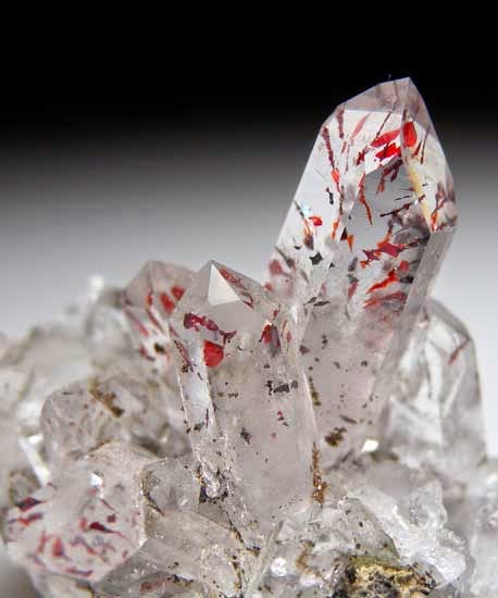
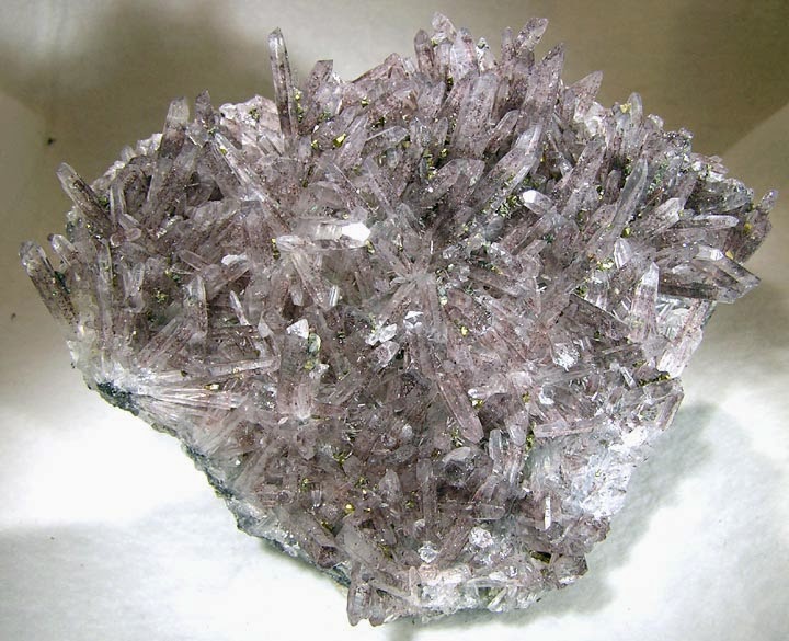
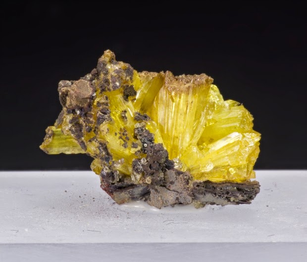
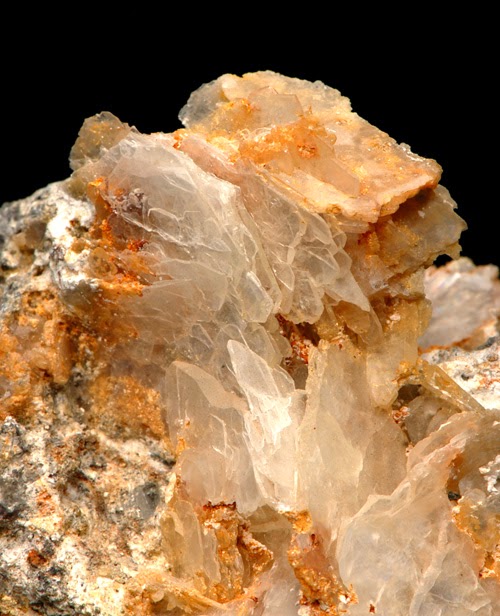
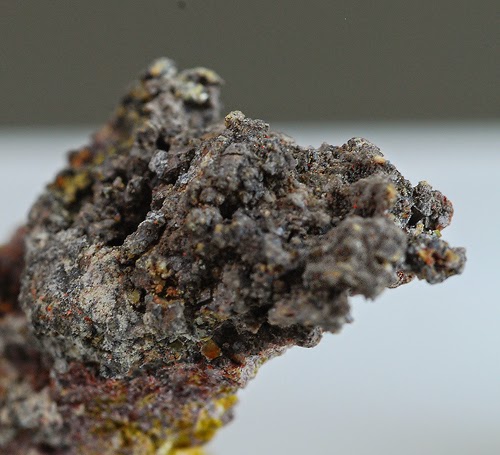
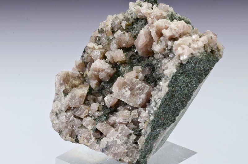
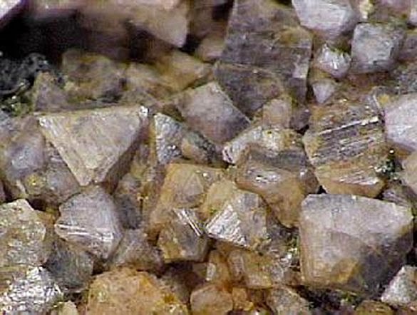
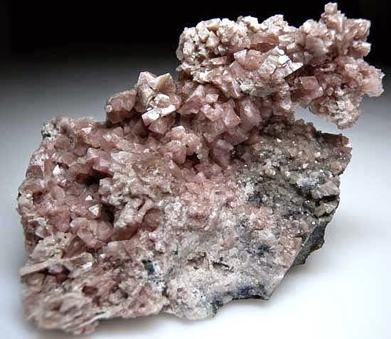
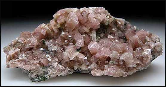
Chemical Formula: γ-FeO(OH) Locality: Common world wide. Name Origin: From the Greek lipis – “scale” and krokis – “fibre.”
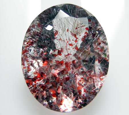
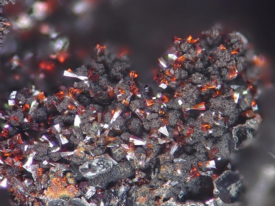
Lepidocrocite (γ-FeO(OH)), also called esmeraldite or hydrohematite, is an iron oxide-hydroxide mineral. Lepidocrocite has an orthorhombic crystal structure, a hardness of 5, specific gravity of 4, a submetallic luster and a yellow-brown streak. It is red to reddish brown and forms when iron-containing substances rust underwater. Lepidocrocite is commonly found in the weathering of primary iron minerals and in iron ore deposits. It can be seen as rust scale inside old steel water pipes and water tanks.
The structure of lepidocrocite is similar to the boehmite structure found in bauxite and consists of layered iron(III) oxide octahedra bonded by hydrogen bonding via hydroxide layers. This relatively weakly bonded layering accounts for the scaley habit of the mineral.
It was first described in 1813 from the Zlaté Hory polymetallic ore deposit in Moravia, Czech Republic. The name is from the Greek lipis for scale and krokis for fibre.
History
Discovery date : 1813 Town of Origin : EISENZECHE, EISERFELD, SIEGEN Country of Origin : ALLEMAGNE
Optical properties
Optical and misc. Properties : Opaque Refractive Index : from 1,94 to 2,51 Axial angle 2V: 83°
Physical Properties
Cleavage: {010} Perfect Color: Red, Yellowish brown, Blackish brown. Density: 4 Diaphaneity: Opaque Fracture: Uneven – Flat surfaces (not cleavage) fractured in an uneven pattern. Hardness: 5 – Apatite Luminescence: Non-fluorescent. Luster: Sub Metallic Streak: dark yellow brown
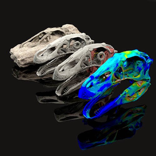
Digital reconstructions of the skull of the dinosaur Erlikosaurus made from a CT scan Credit: Dr Stephan Lautenschlager
New techniques for visualizing fossils are transforming our understanding of evolutionary history according to a paper published by leading palaeontologists at the University of Bristol.
Palaeontology has traditionally proceeded slowly, with individual scientists labouring for years or even decades over the interpretation of single fossils which they have gradually recovered from entombing rock, sand grain by sand grain, using all manner of dental drills and needles.
The introduction of X-ray tomography has revolutionized the way that fossils are studied, allowing them to be virtually extracted from the rock in a fraction of the time necessary to prepare specimens by hand and without the risk of damaging the fossil.
The resulting fossil avatars not only reveal internal and external anatomical features in unprecedented and previously unrealized detail, but can also be studied in parallel by collaborating or competing teams of scientists, speeding up the pace at which evolutionary history is revealed.
These techniques have enabled palaeontologists to move beyond ‘just so stories’, explanations for why sauropod dinosaurs had such long necks, for example, by subjecting digital models of the fossils to biomechanical analysis, including using the same computer techniques that engineers use to design test bridges and aircraft.
However, the scientists from Bristol’s School of Earth Sciences highlight that the potential benefits of fossil avatars are not being realized.
Lead author Dr John Cunningham said: “At a practical level, we simply don’t have the infrastructure for storing and sharing the vast datasets that describe fossils, and the policies of world-leading museums which protect the copyright of fossils are preventing data sharing at a legal level.”
Co-author Dr Stephan Lautenschlager added: “The increasing availability of fossil avatars will allow us to bring long-extinct animals back to life, virtually, by using computer models to work out how they moved and fed. However, in many cases we are hampered by our limited understanding of the biology of the modern species to which we would ideally like to compare the fossils.”
Dr Imran Rahman, also an author of the agenda-setting study, said: “Palaeontologists are making their fossil avatars freely available as files for 3-D printing and so, soon, anyone who wants one, can have a scientifically accurate model of their favourite fossil, for research, teaching, or just for fun!”
Journal Reference:
John A. Cunningham, Imran A. Rahman, Stephan Lautenschlager, Emily J. Rayfield, Philip C.J. Donoghue. A virtual world of paleontology. Trends in Ecology & Evolution, 2014; 29 (6): 347 DOI: 10.1016/j.tree.2014.04.004
Note : The above story is based on materials provided by University of Bristol.
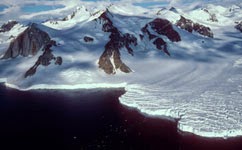
Subglacial lakes in Antarctica might have nutrient-rich groundwater flowing into them, say scientists investigating the origin of the water in ice streams.
Ice streams are huge, fast-flowing glaciers that meander across Antarctica. They are responsible for nearly all of the Antarctic’s contribution to sea-level rise, yet scientists have little understanding of where the water flowing through them comes from. This means that the contents of the subglacial lakes which lie underneath these streams is also a mystery.
The new research, published in Geophysical Research Letters shows for the first time where the water going in and out of these ice streams – their hydrologic budget – comes from.
‘It’s important to understand and quantify the hydrologic budget of these ice streams, as this can control the lubrication and ultimately how fast these ice streams move,’ explains Dr Poul Christoffersen of the Scott Polar Research Institute, lead researcher on the study.
‘Some of these glaciers are slowing, some are speeding up and that’s all in response to changes in the configuration of sources and sinks of water. If we’re trying to understand what they’ll be doing in future we need to understand how they have behaved in the past.’
The team studied five ice streams. They found that the water flowing into them comes mostly from the ice sheet’s deep interior. They also identified a large groundwater reservoir beneath these glacier, which the ice streams draw on to compensate when there is not enough water from the ice sheet to maintain the ice streams fast flow.
The team found that two of the streams moved much faster than three located further south.
‘For two of the ice streams there was a balance between recharge and depletion so they continually flow fast, but for the other three the system doesn’t have enough to provide replenishment, and so they end up losing water. Some are slowing down now, and one stopped altogether about 170 years ago,’ Christoffersen says.
It’s like when water from groundwater reservoirs flow into rivers in England. When an ice stream has little water flowing in from melting ice, the groundwater begins to flow into the stream instead. but unlike England it all happens beneath the ice. If this happens, and there’s lots of groundwater in the network, then the connected subglacial lakes beneath the ice streams are likely to have a a much higher nutrient content, meaning researchers are more likely to find life in them than in the subglacial lakes fed by pure glacial water.
‘Water that’s been stored for thousands of years in the pore spaces of sediments beneath the ice streams are mixing with the water in the subglacial hydrological network. These ancient waters are full of nutrients from the sediment, enough that they could provide life to a thriving microbial habitat,’ explains Christoffersen.
‘A hydrologic system that receives groundwater contributions is much more likely to have high nutrient levels compared to the fast flowing systems which are fed by pure glacial meltwater. That water is pure with very little biochemical material to provide life,’ he says.
More information: Christoffersen, P., M. Bougamont, S. P. Carter, H. A. Fricker, and S. Tulaczyk (2014), “Significant groundwater contribution to Antarctic ice streams hydrologic budget,” Geophys. Res. Lett., 41, 2003-2010, DOI: 10.1002/2014GL059250.
Note : The above story is based on materials provided by PlanetEarth Online
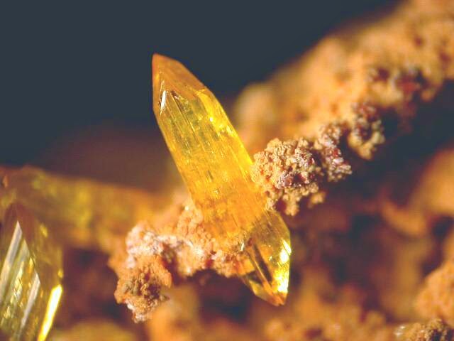
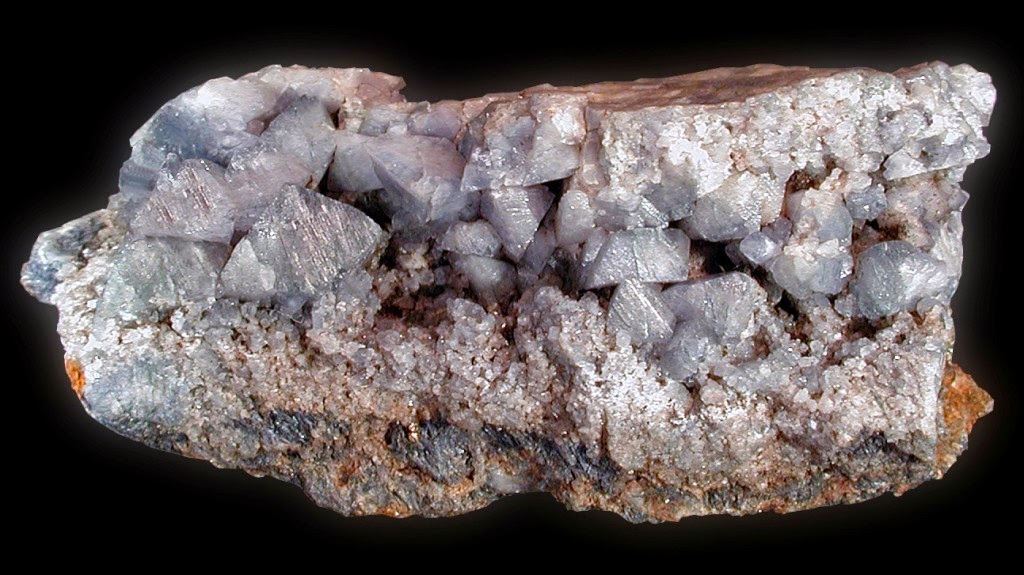
Chemical Formula: Zn2(AsO4)(OH)·H2O Locality: Ojuela mine near Mapimi, Durango. Name Origin: Named after the Belgian mining engineer, Legrande.
Legrandite is a rare zinc arsenate mineral, Zn2(AsO4)(OH)·H2O.
It is an uncommon secondary mineral in the oxidized zone of arsenic bearing zinc deposits and occurs rarely in granite pegmatite. Associated minerals include: adamite, paradamite, kottigite, scorodite, smithsonite, leiteite, renierite, pharmacosiderite, aurichalcite, siderite, goethite and pyrite. It has been reported from Tsumeb, Namibia; the Ojuela mine in Durango, Mexico and at Sterling Hill, New Jersey, USA.
It was first described in 1934 for an occurrence in the Flor de Peña Mine, Nuevo Leon, Mexico and named after M. Legrand, a Belgian mining engineer .
History
Discovery date : 1932 Town of Origin : MINE FLOR DE PENA, LAMPAZOS, NUOVA LEON Country of Origin : MEXIQUE
Optical properties
Optical and misc. Properties : Translucent Refractive Index: from 1,67 to 1,74 Axial angle 2V: 50°
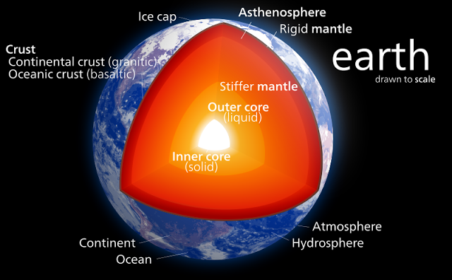
Diagram of the Earth. Credit: Kelvinsong/Wikipeida
Breaking research news from a team of scientists led by Carnegie’s Ho-kwang “Dave” Mao reveals that the composition of the Earth’s lower mantle may be significantly different than previously thought. These results are to be published by Science.
The lower mantle comprises 55 percent of the planet by volume and extends from 670 and 2900 kilometers in depth, as defined by the so-called transition zone (top) and the core-mantle boundary (below). Pressures in the lower mantle start at 237,000 times atmospheric pressure (24 gigapascals) and reach 1.3 million times atmospheric pressure (136 gigapascals) at the core-mantle boundary.
The prevailing theory has been that the majority of the lower mantle is made up of a single ferromagnesian silicate mineral, commonly called perovskite (Mg,Fe)SiO3) defined through its chemistry and structure. It was thought that perovskite didn’t change structure over the enormous range of pressures and temperatures spanning the lower mantle.
Recent experiments that simulate the conditions of the lower mantle using laser-heated diamond anvil cells, at pressures between 938,000 and 997,000 times atmospheric pressure (95 and 101 gigapascals) and temperatures between 3,500 and 3,860 degrees Fahrenheit (2,200 and 2,400 Kelvin), now reveal that iron bearing perovskite is, in fact, unstable in the lower mantle.
The team finds that the mineral disassociates into two phases one a magnesium silicate perovskite missing iron, which is represented by the Fe portion of the chemical formula, and a new mineral, that is iron-rich and hexagonal in structure, called the H-phase. Experiments confirm that this iron-rich H-phase is more stable than iron bearing perovskite, much to everyone’s surprise. This means it is likely a prevalent and previously unknown species in the lower mantle. This may change our understanding of the deep Earth.
“We still don’t fully understand the chemistry of the H-phase,” said lead author Li Zhang, also of Carnegie. “But this finding indicates that all geodynamic models need to be reconsidered to take the H-phase into account. And there could be even more unidentified phases down there in the lower mantle as well, waiting to be identified.”
Scientists from the Magma and Volcanoes Laboratory (CNRS) and the European Synchrotron, the ESRF, have recreated the extreme conditions 600 to 2900 km below the Earth’s surface to investigate the melting of basalt in the oceanic tectonic plates. They exposed microscopic pieces of rock to these extreme pressures and temperatures while simultaneously studying their structure with the ESRF’s extremely powerful X-ray beam.
The results show that basalt produced on the ocean floor has a melting temperature lower than the peridotite which forms the Earth’s mantle. Near the core-mantle boundary, where the temperature rises rapidly, the melting basalt produces liquids rich in silica (SiO2), which react rapidly with the mantle and indicate a speedy dissolution of the basalt back into the depths of the Earth. These experiments provide a new explanation for seismic anomalies at the base of the mantle while fixing its temperature in the region of 4000 K.
The results are published in Science on the 23 May 2014.
The Earth is an active planet. The heat it contains is capable of inducing the mantle convection responsible for plate tectonics. This energy comes from the heat accumulated during the formation of our planet, the latent heat of crystallization of the inner core, and radioactive decay. The temperatures inside the Earth, however, are not well known.
Convection causes hot material to rise to the surface of the Earth and cold material to sink towards the core. Thus, when the ascending mantle begins to melt at the base of the oceanic ridges, the basalt flows along the surface to form what we call the oceanic crust. “Over the course of millennia the crust will then undergo subduction, its greater density causing it to sink into the mantle. This is why the Earth’s continents are known to be several billion years old, while the oldest oceanic crust only dates back 165 million years” said Mohamed Mezouar, scientist at the ESRF.
The temperature at the core-mantle boundary (also known as the D” region) is thought to increase by more than 1000 degrees over a few hundred kilometers, which is significant compared to the temperature gradient across the rest of the mantle. Previous authors have suggested that this temperature rise could cause the partial melting of the mantle, but this hypothesis leaves a number of geophysical observations unexplained. Firstly, the anomalies in the propagation speed of seismic waves do not match those expected for a partial melting of the mantle, and secondly, the melting mantle should lead to the production of liquid pockets in the lowermost mantle, a phenomenon which has never been observed.
The team led by Professor Denis Andrault from the Université Blaise Pascal decided instead to study the melting point of basalt at high depths, and found that it was significantly lower than that of the mantle. The melting of sub-oceanic basalt piles could therefore be responsible for the previously unexplained seismic anomalies. The researchers also showed that the melting basalt generates a liquid rich in SiO2. As the mantle itself contains large quantities of MgO, the interaction of these liquids with the mantle is expected to produce a rapid reaction leading to the formation of the solid MgSiO3 perovskite. This would explain why no liquid pockets have been detected by seismologists in the deep mantle: any streams of liquid should rapidly re-solidify.
If it is indeed the basalt and not the mantle whose melting in the D”-region is responsible for the observed seismic anomalies, then the temperature at the core-mantle boundary must be between 3800 and 4150 Kelvin, between the melting points of basalt and the Earth’s mantle. If this hypothesis is correct, this would be the most accurate determination of the temperature at the core-mantle boundary available today.
“It could solve a long time controversy about the peculiar role of the core-mantle boundary in the dynamical properties of the Earth mantle, said Professor Denis Andrault. ”We know now that the cycle of crust formation at the mid-ocean ridges and crust dissolution in the lowermost mantle may have occured since plate tectonics were active on our planet”, he added.
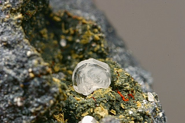
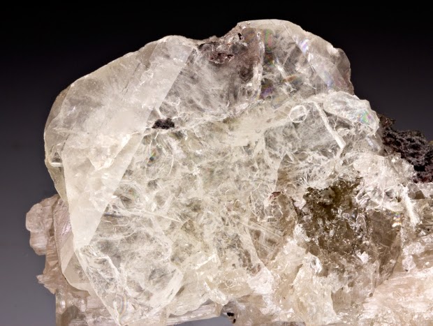
Chemical Formula: Pb4SO4(CO3)2(OH)2 Locality: Leadhills, Lanarkshire, Scotland. Name Origin: Named for the localiy.
Leadhillite is a lead sulfate carbonate hydroxide mineral, often associated with anglesite. It has the formula Pb4SO4(CO3)2(OH)2. Leadhillite crystallises in the monoclinic system, but develops pseudo-hexagonal forms due to crystal twinning. It forms transparent to translucent variably coloured crystals with an adamantine lustre. It is quite soft with a Mohs hardness of 2.5 and a relatively high specific gravity of 6.26 to 6.55.
It was discovered in 1832 in the Susannah Mine, Leadhills in the county of Lanarkshire, Scotland. It is trimorphous with susannite and macphersonite (these three minerals have the same formula, but different structures). Leadhillite is monoclinic, susannite is trigonal and macphersonite is orthorhombic. Leadhillite was named in 1832 after the locality.
Physical Properties
Cleavage: {001} Perfect, {100} Indistinct Color: Colorless, Gray, Yellowish, White, Light blue. Density: 6.26 – 6.55, Average = 6.4 Diaphaneity: Transparent to translucent Fracture: Sectile – Curved shavings or scrapings produced by a knife blade, (e.g. graphite). Hardness: 2.5 – Finger Nail Luminescence: Fluorescent, Short UV=weak gray yellow, Long UV=weak grey yellow. Luster: Adamantine Streak: white
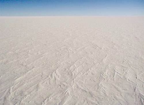
The Antarctic ice sheet. Credit: Stephen Hudson / Wikipedia
A newly-discovered source of oceanic bioavailable iron could have a major impact our understanding of marine food chains and global warming. A UK team has discovered that summer meltwaters from ice sheets are rich in iron, which will have important implications on phytoplankton growth. The findings are reported in the journal Nature Communications on 21st May, 2014.
It is well known that bioavailable iron boosts phytoplankton growth in many of the Earth’s oceans. In turn phytoplankton capture carbon – thus buffering the effects of global warming. The plankton also feed into the bottom of the oceanic food chain, thus providing a food source for marine animals.
The team, comprising researchers from the Universities of Bristol, Leeds, Edinburgh and the National Oceanography Centre, collected meltwater discharged from the 600 km2 Leverett Glacier in Greenland over the summer of 2012, which was subsequently tested for bioavailable iron content. The researchers found that the water exiting from beneath the melting ice sheet contained significant quantities of previously-unconsidered bioavailable iron. This means that the polar oceans receive a seasonal iron boost as the glaciers melt.
Jon Hawkings (Bristol), the lead author, said: “The Greenland and Antarctic Ice Sheets cover around 10% of global land surface. Iron exported in icebergs from these ice sheets have been recognised as a source of iron to the oceans for some time. Our finding that there is also significant iron discharged in runoff from large ice sheet catchments is new. ”
“This means that relatively high iron concentrations are released from the ice sheet all summer, providing a continuous source of iron to the coastal ocean”
Iron is one of the most important biochemical elements, due to its impact on ocean productivity. Despite being the fourth most abundant element in the Earth’s crust, it is mostly not biologically available because it is largely present as unreactive minerals in natural waters. Over the last 20 years there has been controversy over the role of iron in marine food chains and the global carbon cycle, with some groups experimenting with dumping iron into the sea in order to accelerate plankton growth – with the idea that increased plankton growth would capture man made CO2. This work indicates that ice sheets may already be carrying out this process every summer.
Based on their results the team estimates that the flux of bioavailable iron associated with glacial runoff is between 400,000 and 2,500,000 tonnes per year in Greenland and between 60,000 and 100,000 tonnes per year in Antarctica. Taking the combined average figures, this would equal the weight of around 125 Eiffel Towers, or around 3000 fully-laden Boeing 747s being added to the ocean each year.
Jon Hawkings added: “This is a substantial release of iron from the ice sheet, similar in size to that supplied to the oceans by atmospheric dust, another major iron source to the world’s oceans.
At the moment it is just too early to estimate how much additional iron will be carried down from ice sheets into the sea. Of course, the iron release from ice sheet will be localised to the Polar Regions around the ice sheets, so the importance of glacial iron there will be significantly higher. Researchers have already noted that glacial meltwater run-off is associated with large phytoplankton blooms – this may help to explain why”.
Commenting on the relevance of this study, Professor Andreas Kappler (geomicrobiologist at the University of Tübingen, Germany, who is also secretary of the European Association of Geiochemistry) said:
“This study shows that glacier meltwater can contain iron concentrations that are high enough to significantly stimulate biological productivity in oceans that otherwise are oftentimes limited in the element iron that is essential to most living organisms. Although the global importance of this flux of iron into oceans needs to be quantified and the bioavailability of the iron species found should be demonstrated experimentally in future studies, the present study provides a plausible path for nutrient supply to oceanic life.”
More information: Ice sheets as a significant source of highly reactive nanoparticulate iron to the oceans. Authors Jon R. Hawkings, Jemma L. Wadham, Martyn Tranter, Rob Raiswell, Liane G. Benning, Peter J. Statham, Andrew Tedstone, Peter Nienow, Katherine Lee & Jon Telling Nature Communications , 5:3929 , DOI: 10.1038/ncomms4929, published 21 May 2014
Note : The above story is based on materials provided by European Association of Geochemistry
Great ape dietary specialization allowed spread in Eurasia, and also lead to extinction
Newly analyzed tooth samples from the great apes of the Miocene indicate that the same dietary specialization that allowed the apes to move from Africa to Eurasia may have led to their extinction, according to results published May 21, 2014, in the open access journal PLOS ONE by Daniel DeMiguel from the Institut Catalá de Palontologia Miquel Crusafont (Spain) and colleagues.
Apes expanded into Eurasia from Africa during the Miocene (14 to 7 million years ago) and evolved to survive in new habitat. Their diet closely relates to the environment in which they live and each type of diet wears the teeth differently. To better understand the apes’ diet during their evolution and expansion into new habitat, scientists analyzed newly-discovered wearing in the teeth of 15 upper and lower molars belonging to apes from five extinct taxa found in Spain from the mid- to late-Miocene (which overall comprise a time span between 12.3?.2 and 9.7 Ma). They combined these analyses with previously collected data for other Western Eurasian apes, categorizing the wear on the teeth into one of three ape diets: hard-object feeders (e.g., hard fruits, seeds), mixed food feeders (e.g. fruit), and leaf feeders.
Previous data collected elsewhere in Europe and Turkey suggested that the great ape’s diet evolved from hard-shelled fruits and seeds to leaves, but these findings only contained samples from the early-Middle and Late Miocene, while lack data from the epoch of highest diversity of hominoids in Western Europe.
In their research, the scientists found that in contrast with the diet of hard-shelled fruits and seeds at the beginning of the movement of great apes to Eurasia, soft and mixed fruit-eating coexisted with hard-object feeding in the Late Miocene, and a diet specializing in leaves did not evolve. The authors suggest that a progressive dietary diversification may have occurred due to competition and changes in the environment, but that this specialization may have ultimately lead to their extinction when more drastic environmental changes took place.
Citation: DeMiguel D, Alba DM, Moya-Sola S (2014) Dietary Specialization during the Evolution of Western Eurasian Hominoids and the Extinction of European Great Apes. PLoS ONE 9(5): e97442. doi:10.1371/journal.pone.0097442
Note : The above story is based on materials provided by PLOS
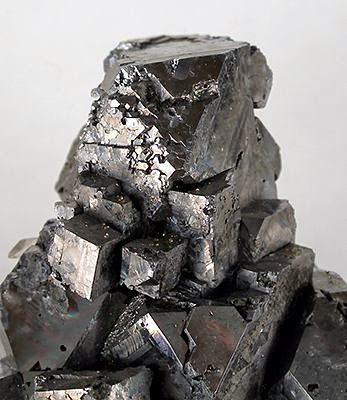
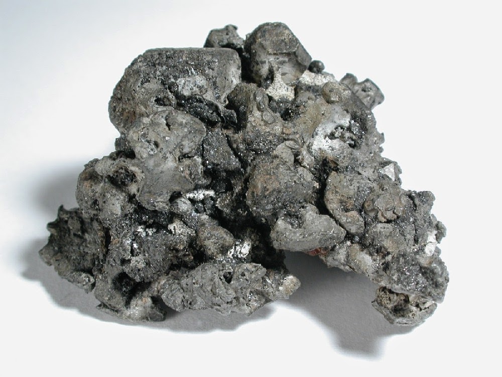
Chemical Formula: Pb Locality: Langban, Sweden. Name Origin: Anglo-Saxon, lead; Latin plumbum.
Lead is a chemical element in the carbon group with symbol Pb and atomic number 82. Lead is a soft and malleable heavy and post-transition metal. Metallic lead has a bluish-white color after being freshly cut, but it soon tarnishes to a dull grayish color when exposed to air. Lead has a shiny chrome-silver luster when it is melted into a liquid. It is also the heaviest non-radioactive element.
Lead is used in building construction, lead-acid batteries, bullets and shot, weights, as part of solders, pewters, fusible alloys, and as a radiation shield. Lead has the highest atomic number of all of the stable elements, although the next higher element, bismuth, has one isotope with a half-life that is so long (over one billion times the estimated age of the universe) that it can be considered stable. Lead’s four stable isotopes have 82 protons, a magic number in the nuclear shell model of atomic nuclei. The isotope lead-208 also has 126 neutrons, another magic number, and is hence double magic, a property that grants it enhanced stability: lead-208 is the heaviest known stable isotope.
If ingested, lead is poisonous to animals and humans, damaging the nervous system and causing brain disorders. Excessive lead also causes blood disorders in mammals. Like the element mercury, another heavy metal, lead is a neurotoxin that accumulates both in soft tissues and the bones. Lead poisoning has been documented from ancient Rome, ancient Greece, and ancient China.
Physical Properties
Cleavage: None Color: Lead gray, Gray white. Density: 11.37 Diaphaneity: Opaque Fracture: Malleable – Deforms rather than breaking apart with a hammer. Hardness: 2-2.5 – Gypsum-Finger Nail Luminescence: Non-fluorescent. Luster: Metallic Magnetism: Nonmagnetic Streak: lead gray
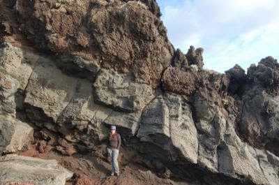
Dr. Rebecca Williams and the remarkable volcanic deposit on Pantelleria island are shown. Credit: Credit: Mike Branney/ University of Leicester
University of Leicester team uncover explosive history of a ‘celebrity hotspot’
A tiny Mediterranean island visited by the likes of Madonna, Sting, Julia Roberts and Sharon Stone is now the focus of a ground-breaking study by University of Leicester geologists.
Pantelleria, a little-known island between Sicily and Tunisia, is a volcano with a remarkable past: 45 thousand years ago, the entire island was covered in a searing-hot layer of green glass.
Volcanologists Drs Mike Branney, Rebecca Williams and colleagues at the University of Leicester Department of Geology have been uncovering previously unknown facts about the island’s physical history.
And their study, published in “Geology” earlier this year, also provides insights into the nature of hazardous volcanic activity in other parts of the world.
Describing the volcanic activity on the island, Dr Branney said: “A ground-hugging cloud of intensely hot gases and volcanic dust spread radially out from the erupting volcano in all directions.
“Incandescent rock fragments suspended in the all-enveloping volcanic cloud were so hot, molten and sticky that they simply fused to the landscape forming a layer of glass, over hills and valleys alike. The hot glass then actually started flowing down all the slopes rather like sticky lava. ‘Ground zero’ in this case was the entire island – nothing would have survived – nature had sterilized and completely enamelled the island.
“Today Pantelleria is verdant and has been re-colonised, but even as you approach it by ferry you can see the green layer of glass covering everything – even sea cliffs look like they’ve been draped in candle wax. Exactly how this happened has only recently come to light.”
The Leicester team have reconstructed how the incandescent density current gradually inundated the entire island. They carefully mapped-out how the chemistry of the glass varies from place to place, and use this to show in unparalleled detail how the ground-hugging current at first was restricted to low, central areas, but then gradually advanced radially towards hills, eventually overtopping them all. Even more remarkably, the devastating current then gradually retreated from hill-tops, and the area covered by it gradually decreased so that, by the end of the eruption, only lower ground, close to the volcano continued to be immersed by it. Such advance-retreat behaviour may be typical of catastrophic currents in nature, such as at other volcanoes, and it may help us better understand undersea currents that are triggered by earthquakes.
“We are trying to ascertain whether this volcanic eruption was just a freak, oddball event. Well, it turns out that the delightful island, now used as a quiet getaway by celebrities, has been the site of at least five catastrophic eruptions of similar type.
“The remarkable volcanic activity on the island was not just a one-off. And as the volcano continues to steam away quite safely, it seems reasonable that in thousands of years time, it may once again erupt with devastating effect.
“Our investigations should help us understand what happens during similar and much larger explosive eruptions elsewhere around the world, such as the Yellowstone–Snake River region of USA”.
Note : The above story is based on materials provided by University of Leicester
Allison Speers, MSU graduate student, works on a fuel cell that can eliminate biodiesel producers’ hazardous wastes and dependence on fossil fuels. Photo by Kurt Stepnitz
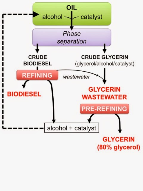
A new fuel-cell concept, developed by an Michigan State University researcher, will allow biodiesel plants to eliminate the creation of hazardous wastes while removing their dependence on fossil fuel from their production process.
The platform, which uses microbes to glean ethanol from glycerol and has the added benefit of cleaning up the wastewater, will allow producers to reincorporate the ethanol and the water into the fuel-making process, said Gemma Reguera, MSU microbiologist and one of the co-authors.
“With a saturated glycerol market, traditional approaches see producers pay hefty fees to have toxic wastewater hauled off to treatment plants,” she said. “By cleaning the water with microbes on-site, we’ve come up with a way to allow producers to generate bioethanol, which replaces petrochemical methanol. At the same time, they are taking care of their hazardous waste problem.”
The results, which appear in the journal Environmental Science and Technology, show that the key to Reguera’s platform is her patented adaptive-engineered bacteria – Geobacter sulfurreducens.
Geobacter are naturally occurring microbes that have proved promising in cleaning up nuclear waste as well in improving other biofuel processes. Much of Reguera’s research with these bacteria focuses on engineering their conductive pili or nanowires. These hair-like appendages are the managers of electrical activity during a cleanup and biofuel production.
MSU is working to eliminate biodiesel producers’ hazardous wastes and dependence on fossil fuels. Courtesy of Gemma Reguera
First, Reguera, along with lead authors and MSU graduate students Allison Speers and Jenna Young, evolved Geobacter to withstand increasing amounts of toxic glycerol. The next step, the team searched for partner bacteria that could ferment it into ethanol while generating byproducts that ‘fed’ the Geobacter.
“It took some tweaking, but we eventually developed a robust bacterium to pair with Geobacter,” Reguera said. “We matched them up like dance partners, modifying each of them to work seamlessly together and eliminate all of the waste.”
Together, the bacteria’s appetite for the toxic byproducts is inexhaustible.
“They feast like they’re at a Las Vegas buffet,” she added. “One bacterium ferments the glycerol waste to produce bioethanol, which can be reused to make biodiesel from oil feedstocks. Geobacter removes any waste produced during glycerol fermentation to generate electricity. It is a win-win situation.”
The hungry microbes are the featured component of Reguera’s microbial electrolysis cells, or MECs. These fuel cells do not harvest electricity as an output. Rather, they use a small electrical input platform to generate hydrogen and increase the MEC’s efficiency even more.
The promising process already has caught the eye of economic developers, who are helping scale up the effort. Through a Michigan Translational Research and Commercialization grant, Reguera and her team are developing prototypes that can handle larger volumes of waste.
Reguera also is in talks with MBI, the bio-based technology “de-risking” enterprise operated by the MSU Foundation, to develop industrial-sized units that could handle the capacities of a full-scale biodiesel plant. The next step will be field tests with a Michigan-based biodiesel manufacturer.
Note : The above story is based on materials provided by Michigan State University
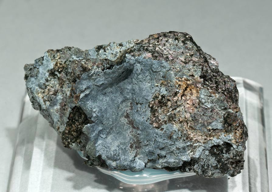
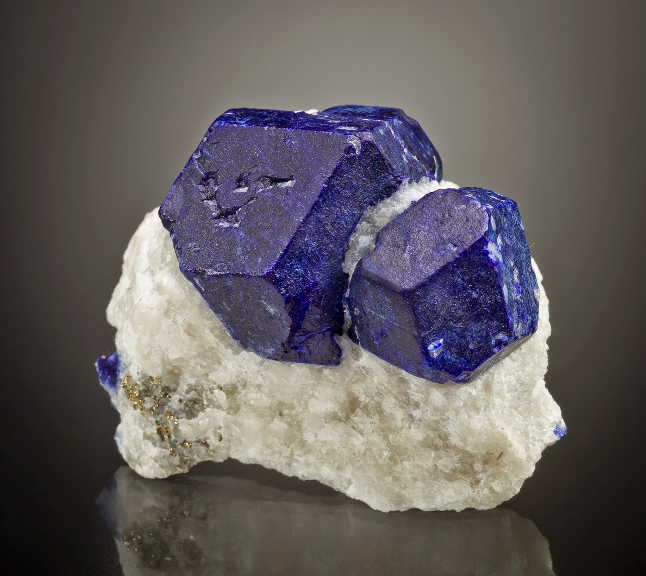
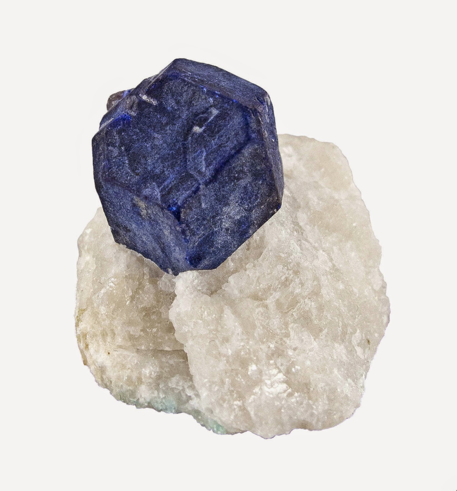
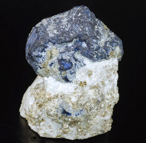
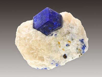
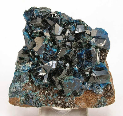
Chemical Formula: (Na,Ca)8[(S,Cl,SO4,OH)2|(Al6Si6O24)] Locality: District of Badakhshan, Afghanistan. Name Origin: From the Persian lazward – “blue.”
Lazurite is a tectosilicate mineral with sulfate, sulfur and chloride with formula: (Na,Ca)8[(S,Cl,SO4,OH)2|(Al6Si6O24)]. It is a feldspathoid and a member of the sodalite group. Lazurite crystallizes in the isometric system although well formed crystals are rare. It is usually massive and forms the bulk of the gemstone lapis lazuli.
Lazurite is a deep blue to greenish blue. The colour is due to the presence of S−3 anions. It has a Mohs hardness of 5.0 to 5.5 and a specific gravity of 2.4. It is translucent with a refractive index of 1.50. It is fusible at 3.5 and soluble in HCl. It commonly contains or is associated with grains of pyrite.
Lazurite is a product of contact metamorphism of limestone and typically is associated with calcite, pyrite, diopside, humite, forsterite, hauyne and muscovite.
History
Discovery date : 1890 Town of Origin : BADAKHSTAN PROV. Country of Origin: AFGHANISTAN
Optical properties
Optical and misc. Properties : Translucent Refractive Index: from 1,50 to 1,52
Physical Properties
Cleavage: {110} Imperfect Color: Blue, Azure blue, Violet blue, Greenish blue. Density: 2.38 – 2.42, Average = 2.4 Diaphaneity: Translucent Fracture: Conchoidal – Fractures developed in brittle materials characterized by smoothly curving surfaces, (e.g. quartz). Hardness: 5.5 – Knife Blade Luminescence: Non-Fluorescent. Luster: Vitreous – Dull Streak: light blue
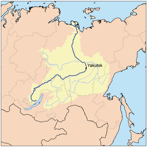
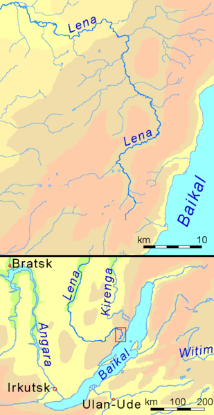
The Lena is the easternmost of the three great Siberian rivers that flow into the Arctic Ocean (the other two being the Ob River and the Yenisei River). It is the 11th longest river in the world and has the 9th largest watershed. It is the largest among the rivers whose watershed is entirely within the Russian territorial boundaries.
Course
Rising at a height of 1,640 metres (5,381 ft) at its source in the Baikal Mountains south of the Central Siberian Plateau, 7 kilometres (4 mi) west of Lake Baikal, the Lena flows northeast, being joined by the Kirenga River, Vitim River and Olyokma River. From Yakutsk it enters the lowlands and flows north until joined by its right-hand tributary the Aldan River. The Verkhoyansk Range deflects it to the north-west; then after receiving its most important left-hand tributary, the Vilyuy River, it makes its way nearly due north to the Laptev Sea, a division of the Arctic Ocean, emptying south-west of the New Siberian Islands by the Lena Delta – 30,000 square kilometres (11,583 sq mi) in area, and traversed by seven principal branches, the most important being the Bykov, farthest east.
Basin
Neighbourhood of the sources of Lena River to Lake Baikal
The total length of the river is estimated at 4,400 km (2,700 mi). The area of the Lena river basin is calculated at 2,490,000 square kilometres (961,394 sq mi). Gold is washed out of the sands of the Vitim and the Olyokma, and mammoth tusks have been dug out of the delta.
Tributaries
The Kirenga River flows north between the upper Lena and Lake Baikal. The Vitim River drains the area northeast of Lake Baikal. The Olyokma River flows north. The Amga River makes a long curve southeast and parallel to the Lena and flows into the Aldan. The Aldan River makes similar curve southeast of the Aldan and flows into the Lena north of Yakutsk. The Maya River, a tributary of the Aldan, drains an area almost to the Sea of Okhotsk. The T-shaped Chona-Vilyuy River system drains most of the area to the west.
History
It is commonly believed that the river Lena derives its name from the original Even-Evenk name Elyu-Ene, which means “the Large River”.
According to folktales related a century after the fact, in the years 1620–23 a party of Russian fur hunters under the leadership of Demid Pyanda sailed up Lower Tunguska, and discovered the proximity of Lena and either carried their boats there or built new ones. In 1623 Pyanda explored some 2,400 kilometers of the river from its upper rocky part to its wide flow in the central Yakutia. In 1628 Vasily Bugor and ten men reached the Lena, collected yasak from the natives and founded Kirinsk in 1632. In 1631 the voyevoda of Yeniseisk sent Pyotr Beketov and twenty men to found an ostrog at Yakutsk (founded in 1632). From Yakutsk other expeditions spread out to the south and east. The Lena delta was reached in 1633.
Baron Eduard Von Toll, accompanied by Alexander von Bunge, carried out an expedition to the Lena delta area and the islands of New Siberia on behalf of the Russian Imperial Academy of Sciences in 1885. They explored the Lena delta with its multitude of arms that flow towards the Arctic Ocean. Then in spring 1886 they investigated the New Siberian Islands and the Yana River and its tributaries. During one year and two days the expedition covered 25,000 km, of which 4,200 km were up rivers, carrying out geodesic surveys en route.
Vladimir Ilyich Ulyanov may have taken his alias, Lenin, from the river Lena, when he was exiled to the Central Siberian Plateau, but the origin of his pen name is uncertain.
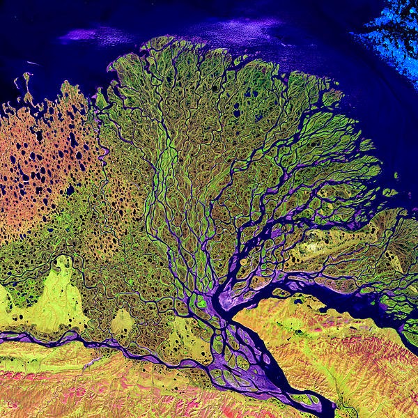
Lena delta
Lena river Delta by Landsat 2000
At the end of the Lena River there is a large delta that extends 100 kilometres (62 mi) into the Laptev Sea and is about 400 km (250 mi) wide. The delta is frozen tundra for about 7 months of the year, but in May transforms the region into a lush wetland for the next few months. Part of the area is protected as the Lena Delta Wildlife Reserve.
The Lena delta divides into a multitude of flat islands. The most important are (from west to east): Chychas Aryta, Petrushka, Sagastyr, Samakh Ary Diyete, Turkan Bel’keydere, Sasyllakh Ary, Kolkhoztakh Bel’keydere, Grigoriy Diyelyakh Bel’kee (Grigoriy Islands), Nerpa Uolun Aryta, Misha Bel’keydere, Atakhtay Bel’kedere, Arangastakh, Urdiuk Pastakh Bel’key, Agys Past’ Aryta, Dallalakh Island, Otto Ary, Ullakhan Ary and Orto Ues Aryta.
Turukannakh-Kumaga is a long and narrow island off the Lena delta’s western shore.
One of the Lena delta islands, Ostrov Amerika-Kuba-Aryta or Ostrov Kuba-Aryta, was named after the island of Cuba during Soviet times. It is on the northern edge of the delta.
Note : The above story is based on materials provided by Wikipedia
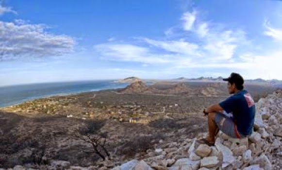
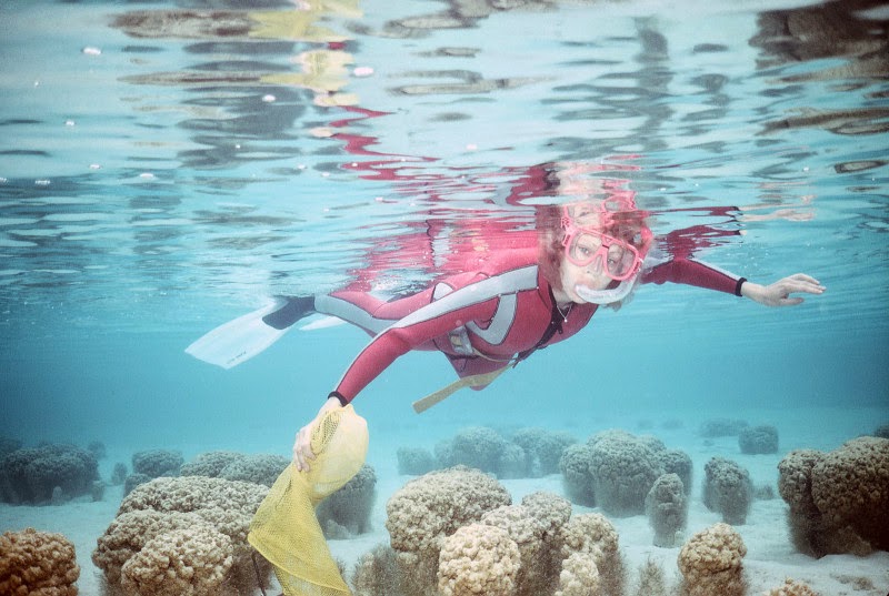
A young man overlooks his home, the coastal community of Cabo Pulmo. Credit: Octavio Aburto.
Cabo Pulmo is a close-knit community in Baja California Sur, Mexico, and the best preserved coral reef in the Gulf of California. But now the lands adjacent to the reef are under threat from a mega-development project, “Cabo Dorado,” should construction go ahead.
Scientists at the University of California, Riverside have published a report on the terrestrial biodiversity of the Cabo Pulmo region that shows the project is situated in an area of extreme conservation value, the center of which is Punta Arena, an idyllic beach setting proposed to be completely cleared to make way for 20,000+ hotel rooms.
“Until recently, the biological value of the lands adjacent to the coral reef of Cabo Pulmo had remained a mystery,” said UC Riverside’s Benjamin Wilder, who helped produce the report. “We now know that these desert lands mirror the tropical waters in importance. This desert-sea ecosystem is a regional biodiversity hotspot.”
According to Wilder, if the Cabo Dorado project proceeds as planned, the regionally endemic plant species and vegetation of Punta Arena will be made extinct.
“Forty-two plants and animals on the Mexican endangered species list would lose critical habitat, two recently described plant species only known from Punta Arena would be lost entirely, and development of the sand dunes of Punta Arena would imperil the most diverse coral reef in the Gulf of California,” he said.
The report resulted from a survey conducted in November 2013 that in just a week’s time documented 560 plants and animals on the land surrounding Cabo Pulmo. The report highlights the unique and ecologically important habitats of the sand spit, Punta Arena, the core zone of the pending development proposal.
The ‘bioblitz’ and resulting report were organized by UCR alum Sula Vanderplank, a biodiversity explorer with the Botanical Research Institute of Texas, and Wilder, a Ph.D. graduate student in the Department of Botany and Plant Sciences, with their advisor Exequiel Ezcurra, a professor of ecology at UCR. The report represents a binational collaboration of 22 scientists from 11 institutions that participated in the expedition and are the top experts on the plants, birds, mammals, and reptiles of Baja California. The survey was organized using the Next Generation of Sonoran Desert Researchers network to assemble a ‘dream-team’ of field biologists.
Ezcurra, the director of UC MEXUS and an acclaimed conservationist, said, “We need to take a careful look at such large scale development projects. Far too many times along the coasts of Mexico we have seen the destruction of areas of great biological importance and subsequent abandonment. By incorporating the natural wealth of the region into development initiatives we can collectively pursue a vision of a prosperous future for our communities that matches the grandeur of the regional landscape.”
In the early 1990s the local community of Cabo Pulmo saw that overfishing was greatly depleting the coral reef ecosystem. The community shifted its local economy to ecotourism and non-extractive livelihoods, and lobbied the Mexican government to make the reef a national park, which was realized in 1995. Since that time there has been a more than 460 percent increase in the total amount of fish in the reserve — the most robust marine reserve in the world.
Wilder, Ezcurra and Vanderplank stress in the report that it is very important that development in this area take into account the inherent limitations of resources, especially fresh water, in a desert setting; the unique habitats found at Punta Arena and the coral reefs of Cabo Pulmo; and, perhaps most important, the local community of Cabo Pulmo.
“We were surprised to see that these desert lands mirrored the biological diversity of the adjacent coral sea,” Wilder said. “Specifically we were not expecting to find such a concentration of rare and endemic taxa in the single region of Punta Arena. This unique biodiversity results from regional geologic forces that were previously un-investigated.
“The bottom line is that the scale of the proposed development, more than 20,000 hotel rooms, is completely disconnected from the ecology of this desert region,” he added. “Any development in the area must account for and sustain the areas natural wealth as well as the local communities of Cabo Pulmo and the nearby town of La Ribera.”
The research team has proposals pending to better understand the linkage between the desert-sea interface of this coastal area. Their aim is to further establish the value of the biological richness of Cabo Pulmo and Punta Arena.
The final report, which based on the scientific results recommends an extension of the Cabo Pulmo National Park to include Punta Arena, was delivered at a public hearing to SEMARNAT, the Mexican federal environmental department. SEMARNAT is expected to make a decision on the future of the Cabo Dorado project by June 15, 2014.
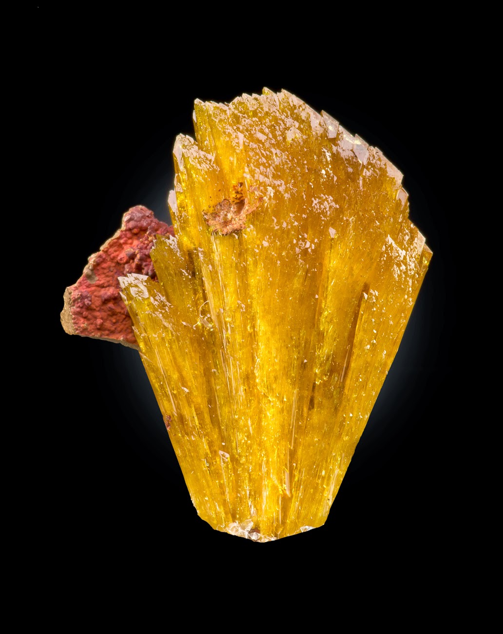
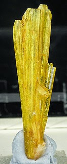
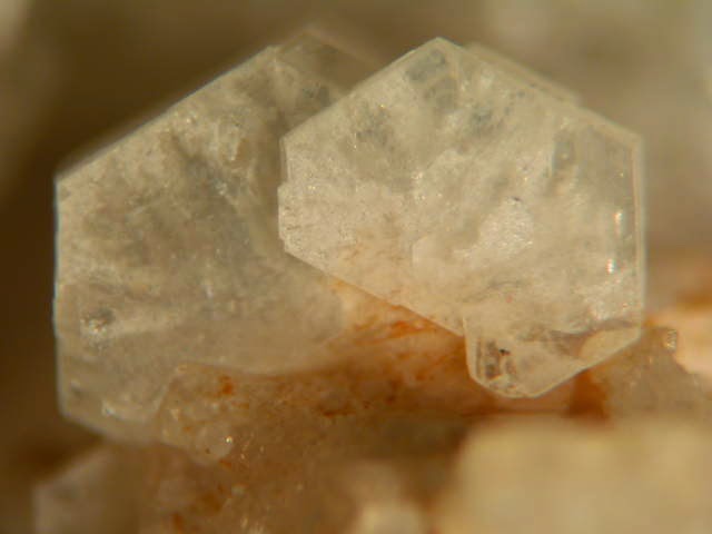
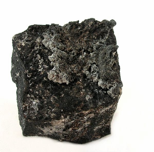
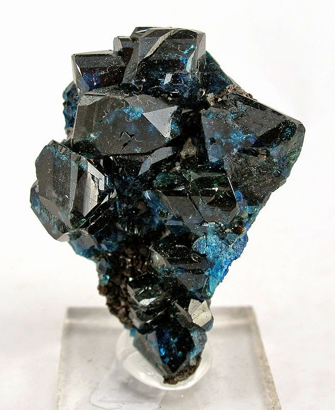
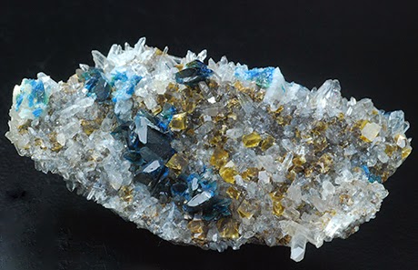
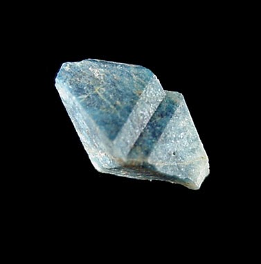
Chemical Formula: (Mg,Fe2+)Al2(PO4)2(OH)2 Locality: Werfen, Salzburg, Austria Name Origin: From the Arabic azul – “sky” and the Greek lithos – “stone.”
Lazulite ((Mg,Fe2+)Al2(PO4)2(OH)2) is a blue, phosphate mineral containing magnesium, iron, and aluminium phosphate. Lazulite forms one endmember of a solid solution series with the darker iron rich scorzalite.
Lazulite crystallizes in the monoclinic system. Crystal habits include steep bipyramidal or wedge-shaped crystals. Lazulite has a Mohs hardness of 5.5 to 6 and a specific gravity of 3.0 to 3.1. It is infusible and insoluble.
History
Discovery date : 1795
Optical properties
Optical and misc. Properties : Subtranslucent to opaque Refractive Index : from 1,61 to 1,64 Axial angle 2V: 69°
Physical Properties
Color: Blue, Blue green, Light blue, Black blue. Density: 3 – 3.1, Average = 3.05 Diaphaneity: Subtranslucent to opaque Fracture: Uneven – Flat surfaces (not cleavage) fractured in an uneven pattern. Hardness: 5-6 – Between Apatite and Orthoclase Luminescence: Non-fluorescent. Luster: Vitreous (Glassy) Streak: white
The late Dr Linda Moore sampling microbialites. Credit: Bob Burne
Scientists have discovered that the earliest living organisms on Earth were capable of making a mineral that may be found on Mars.
The clay-mineral stevensite has been used since ancient times and was used by Nubian women as a beauty treatment, but scientists had believed deposits could only be formed in harsh conditions like volcanic lava and hot alkali lakes.
Researchers led by Dr Bob Burne from the ANU Research School of Earth Sciences have found living microbes create an environment that allows stevensite to form, raising new questions about the stevensite found on Mars.
“It’s much more likely that the stevensite on Mars is made geologically, from volcanic activity,” Dr Burne said.
“But our finding — that stevensite can form around biological organisms — will encourage re-interpretation of these Martian deposits and their possible links to life on that planet.”
Dr Burne and his colleagues from ANU, University of Western Australia and rock imaging company Lithicon, have found microbes can become encrusted by stevensite, which protects their delicate insides and provides the rigidity to allow them to build reef-like structures called “microbialites.”
“Microbialites are the earliest large-scale evidence of life on Earth,” Dr Burne said. “They demonstrate how microscopic organisms are able to join together to build enormous structures that sometimes rivalled the size of today’s coral reefs.”
He said the process still happens today in some isolated places like Shark Bay and Lake Clifton in Western Australia.
“Stevensite is usually assumed to require highly alkaline conditions to form, such as volcanic soda lakes. But our stevensite microbialites grow in a lake less salty than seawater and with near-neutral pH.”
One of the paper’s authors, Dr Penny King from ANU, is a science co-investigator on NASA’s Mars Curiosity rover, which uncovered the presence of possible Martian stevensite.
The findings also have implications for how some of the world’s largest oil reservoirs were formed.
The discovery was made using ANU-developed imaging technology licensed to Lithicon. The data was run on Raijin, the most powerful supercomputer in the Southern Hemisphere, based at the National Computational Infrastructure in Canberra.
Journal Reference:
R. V. Burne, L. S. Moore, A. G. Christy, U. Troitzsch, P. L. King, A. M. Carnerup, P. J. Hamilton. Stevensite in the modern thrombolites of Lake Clifton, Western Australia: A missing link in microbialite mineralization? Geology, 2014; DOI: 10.1130/G35484.1
Note : The above story is based on materials provided by Australian National University.
Professor Francisco J. Rodríguez-Tovar, of the University of Granada, pointing to the bio-event in the late Cretaceous/early Tertiary (when the dinosaurs became extinct) in Agost (Alicante). Credit: Image courtesy of University of Granada
Analysing palaeontological data helps characterize irregular paleoenvironmental cycles, lasting between less than 1 day and more than millions of years.
Francisco J. Rodríguez-Tovar, Professor of Stratigraphy and Paleontology at the University of Granada has shown that the cyclical phenomena that affect the environment, like climate change, in the atmosphere-ocean dynamic and, even, disturbances to planetary orbits, have existed since hundreds of millions of year ago and can be studied by analysing fossils.
This is borne out by the palaeontological data analysed, which have facilitated the characterization of irregular cyclical paleoenvironmental changes, lasting between less than 1 day and up to millions of years.
Francisco J. Rodríguez-Tovar, Professor de Stratigraphy and Paleontology at the University of Granada, has analysed how fossil records can be used as a key tool to characterize these cyclical phenomena that have varying time scales.
The results of this research have been published in the prestigious journal Annual Reviews of Earth and Planetary Sciences, the second-ranked journal in the category of Geosciences, Multidisciplinary in the Journal Citation Reports ranking, after Nature Geosciences, with an impact factor close to 9. Never before has a Spanish scientist succeeded in having an article published in this journal.
As Dr Rodríguez-Tovar indicates, these are cyclical phenomena of a variable scale, from less than a day to more than millions of years, and which have appeared in different ways in the fossil record.
In the case of those lasting between less than 1 day and 1 year, “these are phenomena on an ecological scale essentially associated with variations in tidal and solar cycles that were recorded in the models of growth of organisms like bivalve shells or corals. Hence, we find evidence of them in fossils dating from the Paleozoic (more than 500 million years ago)”, says Prof. Rodríguez-Tovar of the University of Granada.
Moreover, in his article he has studied cyclical phenomena that have lasted between 1 year and 10,000 years, like those associated with the El Niño phenomenon (a cyclical climactic phenomenon causing the warming of South American seas), the so-called Dansgaard-Oeschger Cycles or the Heinrich Events. The latter took place during the last Ice Age, and determined variations in the abundance, distribution and diversity of populations and marine and terrestrial species.
Also, he has analysed cyclical phenomena of between 10 000 and 1 million years ago, essentially associated with climactic changes due to orbital variations (Milankovitch cycles), that are recorded in the evolutionary patterns of specific species, even bringing about their extinction.
Finally, Professor Rodríguez-Tovar has studied cyclical changes lasting over 1 million years, occurring throughout the Phanerozoic period, which are interpretation as being associated with extraterrestrial phenomena (meteorite impacts, such as those occurring in the late Cretaceous/early Tertiary, some 65 million years ago) or terrestrial phenomena (such as large-scale volcanism).
“These changes are related with major periodic extinctions, which affect a high percentage of the biota, since in most cases more than 65% of living organisms became extinct”, Prof. Rodríguez-Tovar points out.
Journal Reference:
Francisco J. Rodríguez-Tovar. Orbital Climate Cycles in the Fossil Record: From Semidiurnal to Million-Year Biotic Responses. Annual Review of Earth and Planetary Sciences, 2013; 42 (1): 140205180347002 DOI: 10.1146/annurev-earth-120412-145922
Note : The above story is based on materials provided by University of Granada.
Chemical Formula: CaAl2(Si2O7)(OH)2·H2O Locality: Reed Station, Tiburon peninsula, Marin County, California, USA. Name Origin: Named for Andrew Cowper Lawson (1861-1952), Scottish-American geologist.
Lawsonite is a hydrous calcium aluminium sorosilicate mineral with formula CaAl2(Si2O7)(OH)2·H2O. Lawsonite crystallizes in the orthorhombic system in prismatic, often tabular crystals. Crystal twinning is common. It forms transparent to translucent colorless, white, and bluish to pinkish grey glassy to greasy crystals. Refractive indices are nα=1.665, nβ=1.672 – 1.676, and nγ=1.684 – 1.686. It is typically almost colorless in thin section, but some lawsonite is pleochroic from colorless to pale yellow to pale blue, depending on orientation. The mineral has a Mohs hardness of 8 and a specific gravity of 3.09. It has perfect cleavage in two directions and a brittle fracture.
Lawsonite is a metamorphic mineral typical of the blueschist facies. It also occurs as a secondary mineral in altered gabbro and diorite. Associate minerals include epidote, titanite, glaucophane, garnet and quartz. It is an uncommon constituent of eclogite.
It was first described in 1895 for occurrences in the Tiburon peninsula, Marin County, California. It was named for geologist Andrew Lawson (1861–1952) of the University of California by two of Lawson’s graduate students, Charles Palache and Frederick Leslie Ransome.
History
Discovery date : 1895 Town of Origin: PENINSULE DE TIBURON, MARIN CO., CALIFORNIE Country of Origin : USA
Optical properties
Optical and misc. Properties: Translucent to transparent Refractive Index: from 1,66 to 1,68 Axial angle 2V : 76-87°