A Dartmouth-led study finds that rising temperatures and ash from Northern Hemisphere forest fires combined to cause large-scale surface melting of the Greenland ice sheet in 1889 and 2012. This contradicts conventional thinking that the melting was driven by warming alone.
The findings suggest that continued climate change will result in nearly annual widespread melting of the ice sheet’s surface by the year 2100. Melting in the dry snow region does not contribute to sea level rise. Instead, the meltwater percolates into the snowpack and refreezes, leaving a less reflective surface. This reformed surface becomes even more susceptible to future melting due to the surface’s reduced reflectance. The ability to reflect sunlight is known as “albedo.”
The study, conducted by Thayer School of Engineering and the Desert Research Institute, is reported in the Proceedings of the National Academy of Sciences. The research was supported by the National Science Foundation and NASA.
“The widespread melting of the Greenland ice sheet required the combination of both of these effects — a lowered snow albedo from ash and unusually warm temperatures — to push the ice sheet over the threshold,” says Kaitlin Keegan, the study’s lead author and a Dartmouth doctoral student. “With both the frequency of forest fires and warmer temperatures predicted to increase with climate change, widespread melt events are likely to happen much more frequently in the future.”
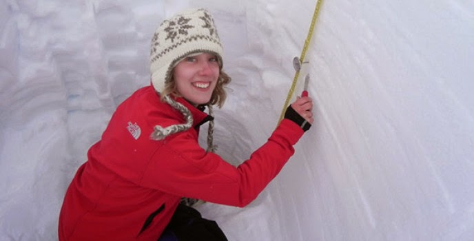
The massive Greenland ice sheet experiences annual melting at low elevations near the coastline, but surface melt is rare in the dry snow region in its center. In July 2012, however, more than 97 percent of the ice sheet experienced surface melt, the first widespread melt during the era of satellite observation. Keegan, who added critical information to NASA’s announcement of the 2012 melt, studies the newly deposited layers of snow that top the 2-mile-thick ice sheet.
In the new study, an analysis of six Greenland shallow ice cores from the dry snow region confirmed that the most recent prior widespread melt occurred in 1889. An ice core from the center of the ice sheet demonstrated that exceptionally warm temperatures combined with black carbon sediments from Northern Hemisphere forest fires reduced albedo below a critical threshold in the dry snow region and caused the large-scale melting events in both 1889 and 2012.
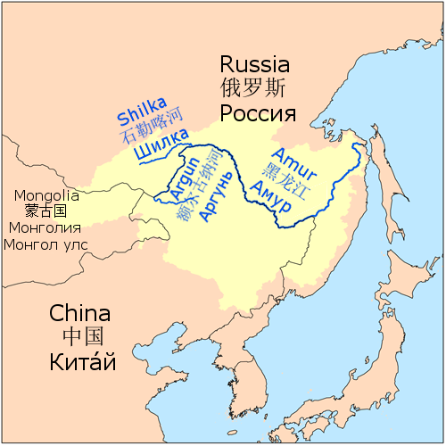
The study did not focus on analyzing the ash to determine the source of the fires, but the presence of a high concentration of ammonium concurrent with the black carbon indicates the ash’s source was large boreal forest fires during the summer in Siberia and North America in June and July 2012. Air masses from these two areas arrived at the Greenland ice sheet’s summit just before the widespread melt event. As for 1889, there are historical records of testimony to Congress of large-scale forest fires in the Pacific Northwest of the United States that summer, but it would be difficult to pinpoint which forest fires deposited ash onto the ice sheet that summer.
The researchers also used Intergovernmental Panel on Climate Change data to project the frequency of widespread surface melting into the year 2100. Since Arctic temperatures and the frequency of forest fires are both expected to rise with climate change, the researchers’ results suggest that large-scale melt events on the Greenland ice sheet may begin to occur almost annually by the end of century. These events are likely to alter the surface mass balance of the ice sheet, leaving the surface susceptible to further melting. The Greenland ice sheet is the second largest ice body in the world after the Antarctic ice sheet.
“Our Earth is a system of systems,” says Thayer Professor Mary Albert, co-author of the study and the director of the U.S. Ice Drilling Program Office. “Improved understanding of the complexity of the linkages and feedbacks, as in this paper, is one challenge facing the next generation of engineers and scientists — people like Kaitlin.”
Note : The above story is based on materials provided by Dartmouth College.