Chemical Formula:Na
2B
4O
6(OH)
2·3(H
2O) Locality: Boron, Kern County, California, the county that contains the fabulous borate deposits at Kramer. Name Origin: Named after it’s locality.
Kernite, also known as rasorite is a hydrated sodium borate hydroxide mineral with formula Na
2B
4O
6(OH)
2·3(H
2O) , It is a colorless to white mineral crystallizing in the monoclinic crystal system typically occurring as prismatic to acicular crystals or granular masses. It is relatively soft with Mohs hardness of 2.5 to 3 and light with a specific gravity of 1.91. It exhibits perfect cleavage and a brittle fracture.
Kernite is soluble in cold water and alters to tincalconite when it dehydrates. It undergoes a non-reversible alteration to metakernite (Na
2B
4O
7·5(H
2O)) when heated to above 100°C.
Occurrence and history
The mineral occurs in sedimentary evaporite deposits in arid regions.
Kernite was discovered in 1926 in eastern Kern County, in Southern California, and later renamed after the county. The location was the US Borax Mine at Boron in the western Mojave Desert. This type material is stored at Harvard University, Cambridge, Massachusetts, and the National Museum of Natural History, Washington, D.C.
The Kern County mine was the only known source of the mineral for a period of time. More recently, kernite is mined in Argentina and Turkey.
The largest documented, single crystal of kernite measured 2.44 x 0.9 x 0.9 m3 and weighed ~3.8 tons.
Physical Properties
Cleavage: {100} Perfect, {001} Perfect, {201} Good Color: Colorless, White. Density: 1.9 – 1.92, Average = 1.91 Diaphaneity: Transparent to translucent Fracture: Brittle – Generally displayed by glasses and most non-metallic minerals. Hardness: 2.5-3 – Finger Nail-Calcite Luminescence: Non-fluorescent. Luster: Vitreous – Pearly Streak: white
Dinosaur phylogeny showing nodes with exceptional rates of body size evolution. Credit: Benson RBJ, Campione NE, Carrano MT, Mannion PD, Sullivan C, et al. (2014) Rates of Dinosaur Body Mass Evolution Indicate 170 Million Years of Sustained Ecological Innovation on the Avian Stem Lineage. PLoS Biol 12(5): e1001853. doi:10.1371/journal.pbio.1001853
Although most dinosaurs went extinct 65 million years ago, one dinosaur lineage survived and lives on today as a major evolutionary success story — the birds.
A study that has ‘weighed’ hundreds of dinosaurs suggests that shrinking their bodies may have helped the group that became birds to continue exploiting new ecological niches throughout their evolution, and become hugely successful today.
An international team, led by scientists at Oxford University and the Royal Ontario Museum, estimated the body mass of 426 dinosaur species based on the thickness of their leg bones. The team found that dinosaurs showed rapid rates of body size evolution shortly after their origins, around 220 million years ago. However, these soon slowed: only the evolutionary line leading to birds continued to change size at this rate, and continued to do so for 170 million years, producing new ecological diversity not seen in other dinosaurs.
A report of the research is published in PLOS Biology.
‘Dinosaurs aren’t extinct; there are about 10,000 species alive today in the form of birds. We wanted to understand the evolutionary links between this exceptional living group, and their Mesozoic relatives, including well-known extinct species like T. rex, Triceratops, and Stegosaurus,’ said Dr Roger Benson of Oxford University’s Department of Earth Sciences, who led the study. ‘We found exceptional body mass variation in the dinosaur line leading to birds, especially in the feathered dinosaurs called maniraptorans. These include Jurassic Park’s Velociraptor, birds, and a huge range of other forms, weighing anything from 15 grams to 3 tonnes, and eating meat, plants, and more omnivorous diets.’
The team believes that small body size might have been key to maintaining evolutionary potential in birds, which broke the lower body size limit of around 1 kilogram seen in other dinosaurs.
‘How do you weigh a dinosaur? You can do it by measuring the thickness of its leg bones, like the femur. This is quite reliable,’ said Dr Nicolás Campione, of the Uppsala University, a member of the team. ‘This shows that the biggest dinosaur Argentinosaurus, at 90 tonnes, was 6 million times the weight of the smallest Mesozoic dinosaur, a sparrow-sized bird called Qiliania, weighing 15 grams. Clearly, the dinosaur body plan was extremely versatile.’
The team examined rates of body size evolution on the entire family tree of dinosaurs, sampled throughout their first 160 million years on Earth. If close relatives are fairly similar in size, then evolution was probably quite slow. But if they are very different in size, then evolution must have been fast.
‘What we found was striking. Dinosaur body size evolved very rapidly in early forms, likely associated with the invasion of new ecological niches. In general, rates slowed down as these lineages continued to diversify,’ said Dr David Evans at the Royal Ontario Museum, who co-devised the project. ‘But it’s the sustained high rates of evolution in the feathered maniraptoran dinosaur lineage that led to birds — the second great evolutionary radiation of dinosaurs.’
The evolutionary line leading to birds kept experimenting with different, often radically smaller, body sizes — enabling new body ‘designs’ and adaptations to arise more rapidly than among larger dinosaurs. Other dinosaur groups failed to do this, got locked in to narrow ecological niches, and ultimately went extinct. This suggest that important living groups such as birds might result from sustained, rapid evolutionary rates over timescales of hundreds of millions of years, which could not be observed without fossils.
‘The fact that dinosaurs evolved to huge sizes is iconic,’ said team member Dr Matthew Carrano of the Smithsonian Institution’s National Museum of Natural History. ‘And yet we’ve understood very little about how size was related to their overall evolutionary history. This makes it clear that evolving different sizes was important to the success of dinosaurs.’
Note : The above story is based on materials provided by University of Oxford.
Scientists have used state-of-the-art imaging techniques to examine the cracks, fractures and breaks in the bones of a 150 million-year-old predatory dinosaur. Credit: Phil Manning
Scientists have used state-of-the-art imaging techniques to examine the cracks, fractures and breaks in the bones of a 150 million-year-old predatory dinosaur.
The University of Manchester researchers say their groundbreaking work – using synchrotron-imaging techniques – sheds new light, literally, on the healing process that took place when these magnificent animals were still alive.
The research, published in the Royal Society journal Interface, took advantage of the fact that dinosaur bones occasionally preserve evidence of trauma, sickness and the subsequent signs of healing.
Diagnosis of such fossils used to rely on the grizzly inspection of gnarled bones and healed fractures, often entailing slicing through a fossil to reveal its cloying secrets. But the synchrotron-based imaging, which uses light brighter than 10 billion Suns, meant the team could tease out the chemical ghosts lurking within the preserved dinosaur bones.
The impact of massive trauma, they discovered, seemed to be shrugged off by many predatory dinosaurs – fossil bones often showed a multitude of grizzly healed injuries, most of which would prove fatal to humans if not medically treated.
Dr Phil Manning, one of the paper’s authors based in Manchester’s School of Earth, Atmospheric and Environmental Sciences, said: “Using synchrotron imaging, we were able to detect astoundingly dilute traces of chemical signatures that reveal not only the difference between normal and healed bone, but also how the damaged bone healed.
“It seems dinosaurs evolved a splendid suite of defence mechanisms to help regulate the healing and repair of injuries. The ability to diagnose such processes some 150 million years later might well shed new light on how we can use Jurassic chemistry in the 21st Century.”
He continued: “The chemistry of life leaves clues throughout our bodies in the course of our lives that can help us diagnose, treat and heal a multitude of modern-day ailments. It’s remarkable that the very same chemistry that initiates the healing of bone in humans also seems to have followed a similar pathway in dinosaurs.”
Co-author Jennifer Anné said: “Bone does not form scar tissue, like a scratch to your skin, so the body has to completely reform new bone following the same stages that occurred as the skeleton grew in the first place. This means we are able to tease out the chemistry of bone development through such pathological studies.
“It’s exciting to realise how little we know about bone, even after hundreds of years of research. The fact that information on how our own skeleton works can be explored using a 150-million-year-old dinosaur just shows how interlaced science can be.”
Professor Roy Wogelius, another co-author from The University of Manchester, added: “It is a fine line when diagnosing which part of the fossil was emplaced after burial and what was original chemistry to the organism. It is only through the precise measurements that we undertake at the Diamond Synchrotron Lightsource in the UK and the Stanford Synchrotron Lightsource in the US that we were able to make such judgments.”
Note : The above story is based on materials provided by Manchester University.
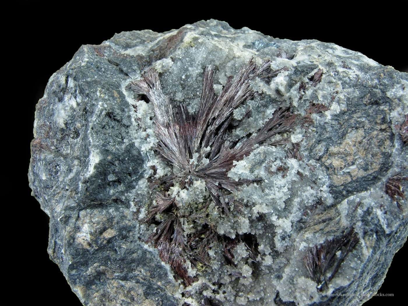
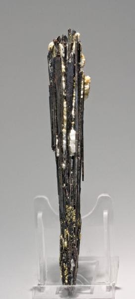
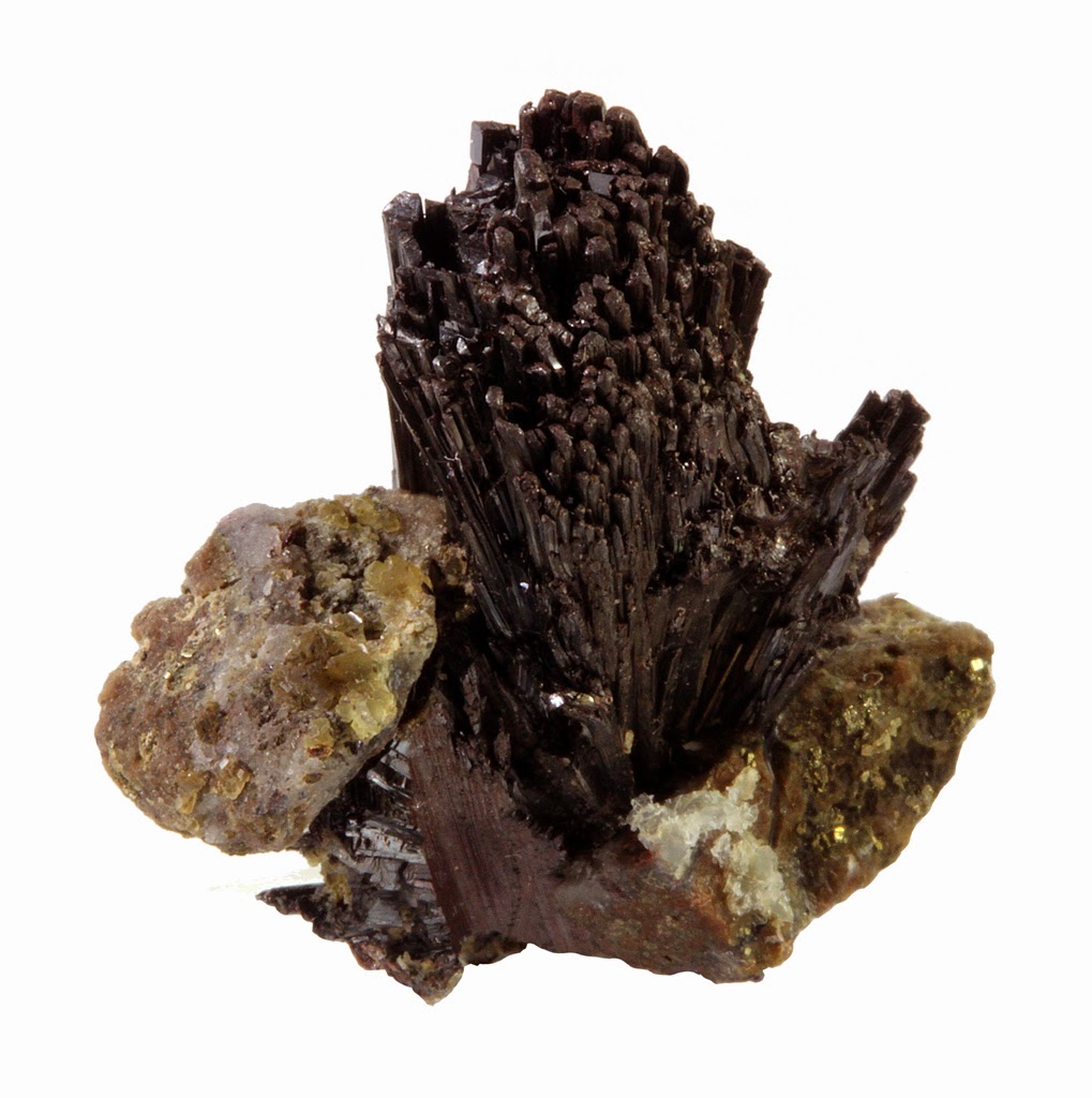
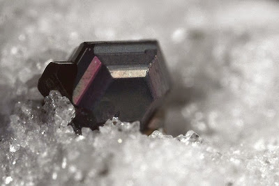
Chemical Formula: Sb2S2O Locality: Braunsdorf, near Freiberg, Saxony, Germany. Name Origin: Name from kermes, a name given from the Persian qurmizq, “crimson” in the older chemistry to red amorphous antimony trisulphide, often mixed with antimony trioxide.Kermesite or antimony oxysulfide is also known as red antimony (Sb2S2O) . The mineral’s color ranges from cherry red to a dark red to a black. Kermesite is the result of partial oxidation between stibnite (Sb2S3)) and other antimony oxides such as valentinite (Sb2O3) or stibiconite (Sb3O6(OH)). Under certain conditions with oxygenated fluids the transformation of all sulfur to oxygen would occur but kermesite occurs when that transformation is halted.
Physical Properties
Cleavage: {100} Perfect Color: Violet red, Cherry red, Red. Density: 4.5 – 4.6, Average = 4.55 Diaphaneity: Translucent to Opaque Fracture: Brittle – Generally displayed by glasses and most non-metallic minerals. Hardness: 1.5-2 – Talc-Gypsum Luminescence: Non-fluorescent. Luster: Adamantine Magnetism: Nonmagnetic Streak: brownish red
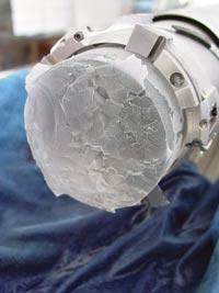
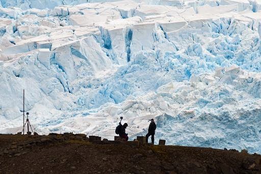
Ice core in the drill head. Past variations of local surface temperatures in polar regions are reconstructed by analysing ice cores drilled in Greenland and Antarctica. Credit: Laurent Augustin
Analysis of data collected from ice cores and marine sediment cores in both polar regions has given scientists a clearer picture of how the Earth’s climate changed during the last Interglacial period. This comparatively warm time period occurred between 130,000 and 115,000 years ago.
By lining up the records, and establishing a common chronology, Dr Emilie Capron, from British Antarctic Survey, concluded that Antarctica was a few degrees warmer than it is today and that the Southern Hemisphere warmed earlier than the Northern Hemisphere.
Results from her findings have been presented to the European Geosciences Union General Assembly in Vienna, Austria this week (27th April – 2nd May 2014).
Dr. Capron said: “To understand our changing climate we need to go back in time. Past warm periods, called interglacials, are particularly interesting because they provide insights as to how current natural changes may interact with those originating from human influences.”
The results, which have been submitted to a science journal for publication, will help climate modellers predict future climate change. Questions remain about the contribution Antarctic and Greenland glaciers may make towards sea level rise.
Dr Capron’s results not only confirm the last interglacial period was warmer than today but also that surface temperature peaks weren’t uniform across the globe.
Data from more than forty cores were examined as part of the research project.
The work is part of a broad ranging interdisciplinary programme, the iGlass consortium, which integrates new field data, data synthesis and numerical modelling, in order to study the response of ice volume and sea level to different climatic states during the last five interglacial periods.
Over the last 1 million years, the Earth’s climate has alternated between warm interglacial periods and cold glacial periods characterised by the growth of ice sheets in the northern hemisphere. Interglacials re-occur roughly every 100,000 years between ice ages. The present interglacial began around 10,000 years ago and has been relatively stable since then.
Note : The above story is based on materials provided by British Antarctic Survey
File photo taken in March 2014 shows scientists work at the Comandante Ferraz base in Antarctica
Polar scientists said Thursday they had successfully drilled a 2,000-year-old ice core in the heart of Antarctica in a bid to retrieve a frozen record of how the planet’s climate has evolved.
The Aurora Basin North project involves scientists from Australia, China, France, Denmark, Germany and the United States who hope it will also advance the search for the scientific “holy grail” of the million-year-old ice core.
The five-week expedition, in a hostile area that harbours some of the deepest ice in the frozen continent, over three kilometres (1.9-miles) thick, will give experts access to some of the most detailed records yet of past climate in the vast region.
About two tonnes of ice core sections drilled at Aurora Basin, 500 kilometres (310 miles) inland of Australia’s Casey station, is now being distributed to Australian and international ice core laboratories.
They will conduct an analysis of atmospheric gases, particles and other chemical elements that were trapped in snow as it fell and compacted to form ice.
Australian Antarctic Division glaciologist and project leader Mark Curran said it will help fill a gap in the science community’s knowledge of climate records.
“Using a variety of scientific tests on each core, we’ll be able to obtain information about the temperature under which the ice formed, storm events, solar and volcanic activity, sea ice extent, and the concentration of different atmospheric gases over time,” he said.
The team, working in temperatures of minus 30 Celsius, used a Danish Hans Tausen drill to extract the main 303-metre-long ice core, which will provide annual climate records for the past 2,000 years.
“There are only a handful of records with comparable resolution that extend to 2,000 years from the whole of Antarctica, and this is only the second one from this sector of East Antarctica,” added Curran.
Additionally two smaller drills were used to take out 116 and 103-metre cores spanning the past 800 to 1,000 years.
Data collected during the drill should help scientists locate a suitable site for a more ambitious expedition to collect a one million year-old ice core in the future.
“Such an ice core would help us understand what caused a dramatic shift in the frequency of ice ages about 800,000 years ago, and further understand the role of carbon dioxide in climate change,” said Curran.
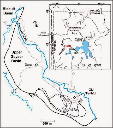
This is a map showing the location of Daisy and Old Faithful geysers in Yellowstone’s Upper Geyser Basin. Inset map of Yellowstone National Park shows the weather station at Yellowstone Lake, seismic stations LKWY and H17A, and strainmeter B944. Credit: Journal of Geophysical Research: Solid Earth, DOI:10.1002/2013JB010803
The intervals between geyser eruptions depend on a delicate balance of underground factors, such as heat and water supply, and interactions with surrounding geysers. Some geysers are highly predictable, with intervals between eruptions (IBEs) varying only slightly. The predictability of these geysers offer earth scientists a unique opportunity to investigate what may influence their eruptive activity, and to apply that information to rare and unpredictable types of eruptions, such as those from volcanoes.
Dr. Shaul Hurwitz took advantage of a decade of eruption data—spanning from 2001 to 2011—for two of Yellowstone’s most predictable geysers, the cone geyser Old Faithful and the pool geyser, Daisy.
Dr. Hurwitz’s team focused their statistical analysis on possible correlations between the geysers’ IBEs and external forces such as weather, earth tides and earthquakes. The authors found no link between weather and Old Faithful’s IBEs, but they did find that Daisy’s IBEs correlated with cold temperatures and high winds. In addition, Daisy’s IBEs were significantly shortened following the 7.9 magnitude earthquake that hit Alaska in 2002.
The authors note that atmospheric processes exert a relatively small but statistically significant influence on pool geysers’ IBEs by modulating heat transfer rates from the pool to the atmosphere. Overall, internal processes and interactions with surrounding geysers dominate IBEs’ variability, especially in cone geysers.
More information: Shaul Hurwitz, Robert A. Sohn, Karen Luttrell, Michael Manga, “Triggering and modulation of geyser eruptions in Yellowstone National Park by earthquakes, earth tides, and weather”, Journal of Geophysical Research: Solid Earth, DOI: 10.1002/2013JB010803
Note :The above story is based on materials provided by Wiley
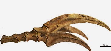
Fossil of the enlarged claws on the forelimbs of Therizinosaurus cheloniformes Credit: Dr Stephan Lautenschlager
How claw form and function changed during the evolution from dinosaurs to birds is explored by a new University of Bristol study into the claws of a group of theropod dinosaurs known as therizinosaurs.
Theropod dinosaurs, a group which includes such famous species as Tyrannosaurus rex and Velociraptor, are often regarded as carnivorous and predatory animals, using their sharp teeth and claws to capture and dispatch prey. However, a detailed look at the claws on their forelimbs revealed that the form and shape of theropod claws are highly variable and might also have been used for other tasks.
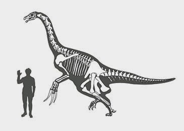
Therizinosaurs were very large animals, up to 7m tall Credit: Dr Stephan Lautenschlager
Inspired by this broad spectrum of claw morphologies, Dr Stephan Lautenschlager from Bristol’s School of Earth Sciences studied the differences in claw shape and how these are related to different functions.
His research focussed on the therizinosaurs, an unusual group of theropods which lived between 145 and 66 million years ago. Therizinosaurs were very large animals, up to 7m tall, with claws more than 50cm long on their forelimbs, elongated necks and a coat of primitive, down-like feathers along their bodies. But in spite of their bizarre appearance, therizinosaurs were peaceful herbivores.
Dr Lautenschlager said: “Theropod dinosaurs were all bipedal, which means their forelimbs were no longer involved in walking as in other dinosaurs. This allowed them to develop a whole new suite of claw shapes adapted to different functions.”
In order to fully understand how these different claws on the forelimbs were used, detailed computer models were created to simulate a variety of possible functions for different species and claw morphologies.
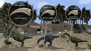
Illustration showing different claw shapes in therizinosaur dinosaurs and the adaptation to specific functions Credit: Dr Stephan Lautenschlager
The dinosaur claws were also compared to the claws of mammals, still alive today, whose function (that is, how and for what the claws are used) is already known.
In the course of evolution, several theropod groups, including therizinosaurs, changed from being carnivores to become plant-eaters. This new study reveals that, during this transition, theropod dinosaurs developed a large variety of claw shapes adapted to specific functions, such as digging, grasping or piercing.
Dr Lautenschlager said: “It’s fascinating to see that, with the shift from a carnivorous to a plant-based diet, we find a large variety of claw shapes adapted to different functions. This suggests that dietary adaptations were an important driver during the evolution of theropod dinosaurs and their transition to modern birds.”
Note : The above story is based on materials provided by University of Bristol.
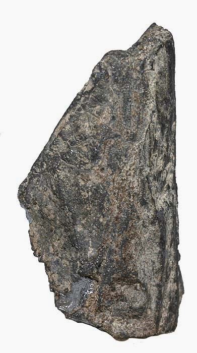
Chemical Formula: Pb14(As,Sb)6S23 Locality: Binnental, Valais, Switzerland. Name Origin: Named after H. Jordan from Saarbrucken.
Jordanite is a sulfosalt mineral with chemical formula Pb14(As,Sb)6S23 in the monoclinic crystal system, named after the German scientist Dr H. Jordan (1808–1887) who discovered it in 1864.
Lead-grey in colour (frequently displaying an iridescent tarnish), its streak is black and its lustre is metallic. Jordanite has a hardness of 3 on Mohs scale, has a density of approximately 6.4, and a conchoidal fracture.
The type locality is the Lengenbach Quarry in the Binn Valley, Wallis, Switzerland.
Physical Properties
Cleavage: {010} Distinct Color: Lead gray. Density: 5.5 – 6.4, Average = 5.95 Diaphaneity: Opaque Fracture: Brittle – Conchoidal – Very brittle fracture producing small, conchoidal fragments. Hardness: 3 – Calcite Luster: Metallic Streak: black
The image shows two Qianzhousaurus individuals hunting. The one in the foreground is chasing a small feathered dinosaur called Nankangia and the one in the background is eating a lizard. Fossils of these three species are known from the ca. 72-66 million-year-old site in Ganzhou, China, where Qianzhousaurus was found. Credit: Chuang Zhao
Scientists have discovered a new species of long-snouted tyrannosaur, nicknamed Pinocchio rex, which stalked Earth more than 66 million years ago.
Researchers say the animal, which belonged to the same dinosaur family as Tyrannosaurus rex, was a fearsome carnivore that lived in Asia during the late Cretaceous period.
The newly found ancient predator looked very different from most other tyrannosaurs. It had an elongated skull and long, narrow teeth compared with the deeper, more powerful jaws and thick teeth of a conventional T. rex.
Palaeontologists were uncertain of the existence of long-snouted tyrannosaurs until the remains of the dinosaur — named Qianzhousaurus sinensis — were unearthed in southern China.
Until now, only two fossilised tyrannosaurs with elongated heads had been found, both of which were juveniles. It was unclear whether these were a new class of dinosaur or if they were at an early growth stage, and might have gone on to develop deeper, more robust skulls.
The new specimen, described by scientists from the Chinese Academy of Geological Sciences and the University of Edinburgh, is of an animal nearing adulthood. It was found largely intact and remarkably well preserved, thereby confirming the existence of tyrannosaur species with long snouts.
Experts say Qianzhousaurus sinensis lived alongside deep-snouted tyrannosaurs but would not have been in direct competition with them, as they were larger and probably hunted different prey.
Following the find, researchers have created a new branch of the tyrannosaur family for specimens with very long snouts, and they expect more dinosaurs to be added to the group as excavations in Asia continue to identify new species.
Qianzhousaurus sinensis lived until around 66 million years ago when all of the dinosaurs became extinct, likely as the result of a deadly asteroid impact.
Findings from the study, funded by the Natural Science Foundation of China and the National Science Foundation, are published in the journal Nature Communications.
Dr Steve Brusatte, of the University of Edinburgh’s School of GeoSciences, and one of the authors of the study, said: “This is a different breed of tyrannosaur. It has the familiar toothy grin of T. rex, but its snout was much longer and it had a row of horns on its nose. It might have looked a little comical, but it would have been as deadly as any other tyrannosaur, and maybe even a little faster and stealthier.”
Professor Junchang Lü, of the Institute of Geology, Chinese Academy of Geological Sciences, said: “The new discovery is very important. Along with Alioramus from Mongolia, it shows that the long-snouted tyrannosaurids were widely distributed in Asia. Although we are only starting to learn about them, the long-snouted tyrannosaurs were apparently one of the main groups of predatory dinosaurs in Asia.”
Note : The above story is based on materials provided by University of Edinburgh.
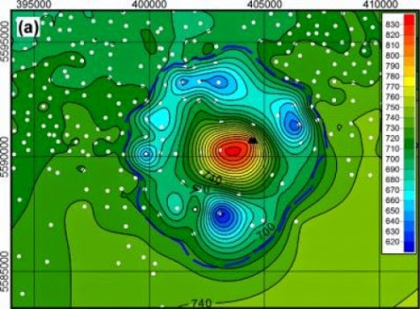
This is a map showing the structure and contour of the Bow City crater. Color variation shows meters above sea level. Credit: Alberta Geographic Survey/University of Alberta
The discovery of an ancient ring-like structure in southern Alberta suggests the area was struck by a meteorite large enough to leave an eight-kilometre-wide crater, producing an explosion strong enough to destroy present-day Calgary, say researchers from the Alberta Geological Survey and University of Alberta.
The first hints about the impact site near the southern Alberta hamlet of Bow City were discovered by a geologist with the Alberta Geological Survey and studied by a U of A team led by Doug Schmitt, Canada Research Chair in Rock Physics.
Time and glaciers have buried and eroded much of the evidence, making it impossible at this point to say with full certainty the ring-like structure was caused by a meteorite impact, but that’s what seismic and geological evidence strongly suggests, said Schmitt, a professor in the Faculty of Science and co-author of a new paper about the discovery.
“We know that the impact occurred within the last 70 million years, and in that time about 1.5 km of sediment has been eroded. That makes it really hard to pin down and actually date the impact.”
Erosion has worn away all but the “roots” of the crater, leaving a semicircular depression eight kilometres across with a central peak. Schmitt says that when it formed, the crater likely reached a depth of 1.6 to 2.4 km — the kind of impact his graduate student Wei Xie calculated would have had devastating consequences for life in the area.
“An impact of this magnitude would kill everything for quite a distance,” he said. “If it happened today, Calgary (200 km to the northwest) would be completely fried and in Edmonton (500 km northwest), every window would have been blown out. Something of that size, throwing that much debris in the air, potentially would have global consequences; there could have been ramifications for decades.”
The impact site was first discovered in 2009 by geologist Paul Glombick, who at the time was working on a geological map of the area for the Alberta Geological Survey. Glombick relied on existing geophysical log data from the oil and gas industry when he discovered a bowl-shaped structure.
The Alberta Geological Survey contacted the U of A and Schmitt to explore further, peeking into Earth by analyzing seismic data donated by industry. Schmitt’s student, Todd Brown, later confirmed a crater-like structure.
Note : The above story is based on materials provided by University of Alberta.
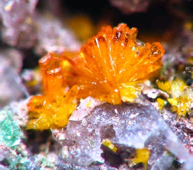
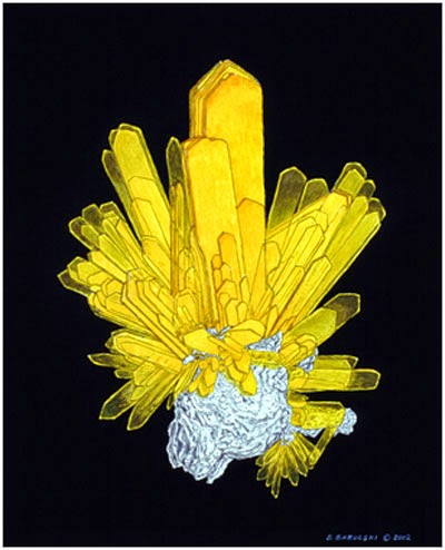
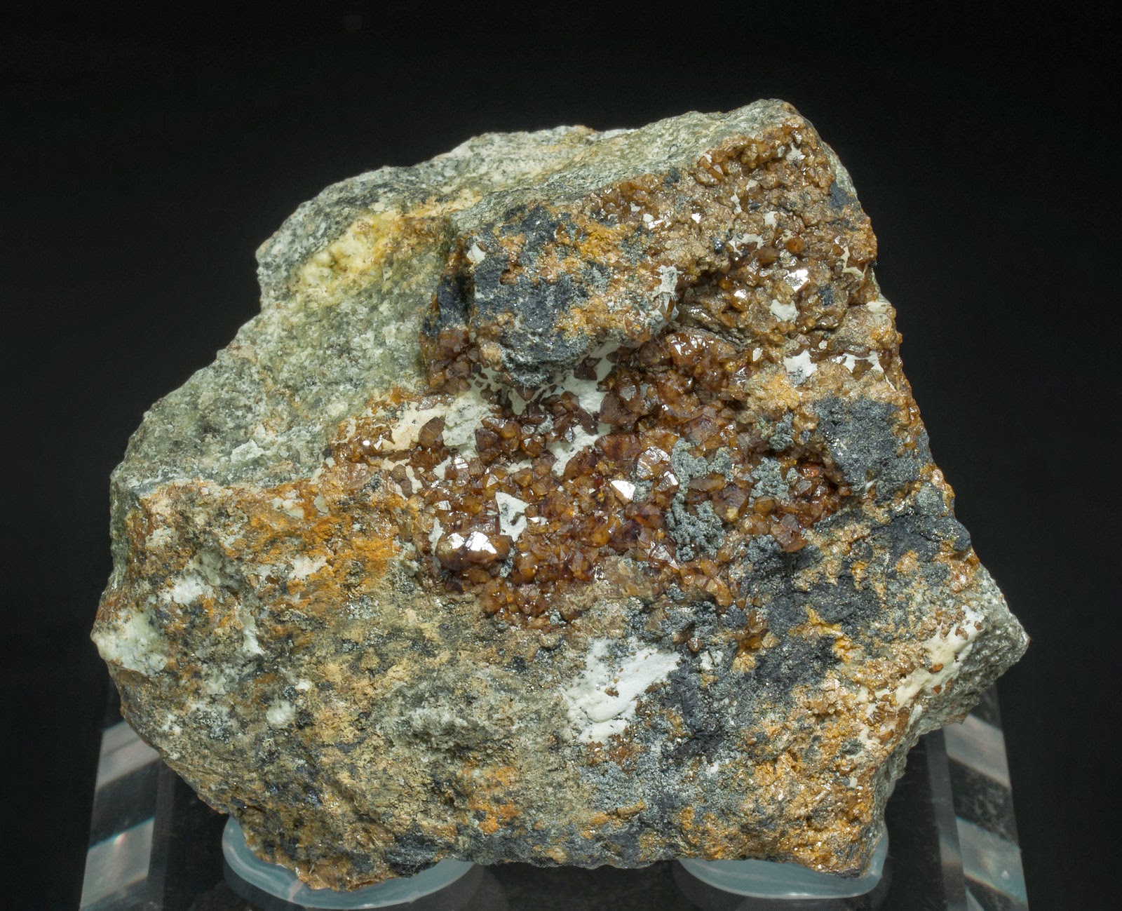
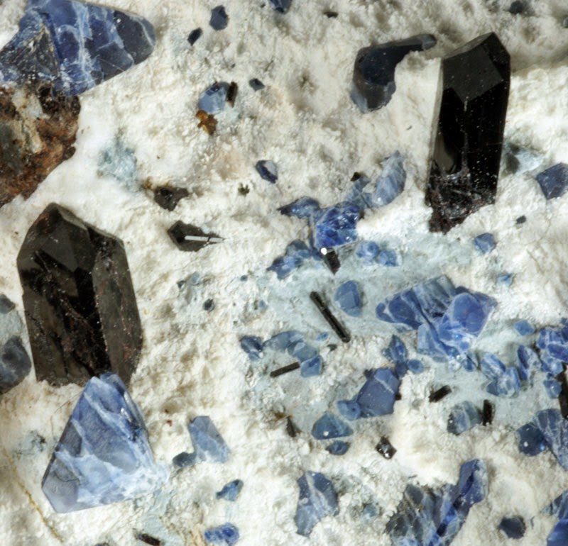
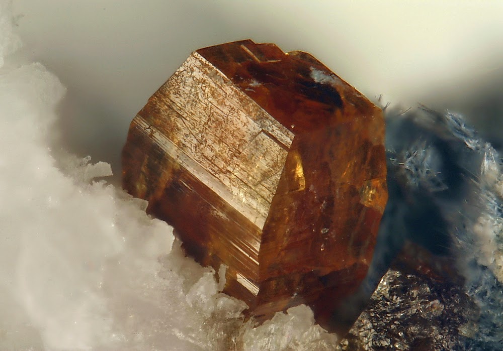
Chemical Formula: NaBa2Ce2FeTi2[Si4O12]2O2(OH,F)·H2O Locality: Benitoite Gem mine, head waters of the San Benito River, Joaquin Ridge, Diablo Range, 1 mile south of Santa Rita Peak, San Benito Co. California. Name Origin: Named after its locality.
Joaquinite, which was discovered in 1909, is a pretty rare mineral. It is most renown for its association with other exotic minerals such as the sapphire blue benitoite, the red-black neptunite and the snow white natrolite. If it were not for these minerals which are found in San Benito County, California; joaquinite might not be so well known. It forms typically small, sparkling, brown to yellow, well formed crystals usually scattered on massive green serpentine.
Joaquinite is a product of some very unusual hydrothermal solutions. These solutions contained the elements titanium, niobium, lithium, barium, niobium, manganese, fluorine, cerium and several others. Anyone of them by themselves is not that unusual, but together in one solution and in such high concentrations is quite unusual. How they came to be combined like this is not yet well understood, but their product of unusual silicate minerals is much appreciated.
Physical Properties
Cleavage: Good Color: Brown, Honey yellow, Orange. Density: 3.62 – 3.98, Average = 3.8 Diaphaneity: Transparent to Translucent Fracture: Brittle – Generally displayed by glasses and most non-metallic minerals. Hardness: 5-5.5 – Apatite-Knife Blade Luminescence: Non-fluorescent. Luster: Vitreous (Glassy)
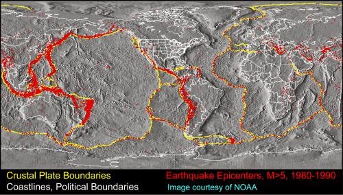
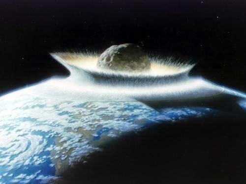
A rock the size of a small city hurtles towards Earth, smashing a crater bigger than the span between Washington, D.C. and New York City. The heat and shockwave raises the temperature of the atmosphere above boiling as huge seismic waves ripple through the Earth’s crust.
New research indicates that such an impact may have happened to our planet, although (thankfully) it was long before civilization arose. About 3.26 billion years ago, an object between 23 and 26 miles wide (37 and 58 kilometers) crashed into the Earth somewhere and left geological evidence behind in South Africa. Surprisingly, the impact may have made the Earth a friendlier place for life because it corresponds with this planet’s establishment of plate tectonics.
Finding the crater, though, is likely an impossible task. There are few rocks of this age on the entire Earth, the notable exception being the nearly 4-billion-old Canadian Shield that stretches across much of eastern Canada. Little remains of that era of history, making it necessary for researchers to do detective work to learn more about the impactor.
“It’s like the aftermath of a tornado where the insurance company won’t pay because your car was sucked off of your driveway and you can’t find the car, so they can’t pay it,” said Norm Sleep, a geophysicist at Stanford University who led the research. “You don’t know if it was stolen or damaged or wrecked or whatever because you can’t find it. We have the same difficulty.”
Sleep and departmental co-author Donald Lowe published their research in the journal Geochemistry, Geophysics and Geosystems in April. The paper is called “Physics of crustal fracturing and chert dike formation triggered by asteroid impact, ∼3.26 Ga, Barberton greenstone belt, South Africa.”
Starting up plate tectonics?
The only life in that era was microbial, although Lowe pointed out they would have struggled with their new circumstances. “To say the least, it would have adversely affected life near the surface,” he said.
While whole microbe communities could have been wiped out, on the species level many would have survived. Life was all over the Earth and not just in the area of the impact, and microbes are better able to withstand sudden temperature changes than more advanced lifeforms.
Perhaps microbes would have suffered after the impact, but in its wake, the impactor could have helped change our planet into one that better supports complex life. Lowe pointed out that plate tectonics seems to have appeared around 3 billion to 3.2 billion years ago, around the same time the impactor smashed into the Earth.
Huge as it was, the impactor was probably too small to have affected plate tectonics all over the Earth, said Lowe and Sleep. In the local area, however, it could have caused great upheaval. Moreover, the impactor crashed into the Earth during an era known as the Late Heavy Bombardment, when rocks and comets smashed into our planet and all the other ones. The Moon still bears scars from that time. The Earth’s have eroded away, but the effects may still linger.
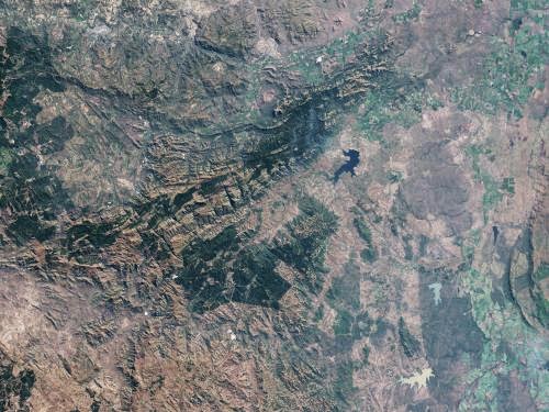
The Barberton Greenstone Belt in South Africa. Credit: Jesse Allen/Landsat/USGS
If enough big objects hit the Earth frequently enough, it could have broken up the primitive plate structure on our planet into the plate tectonics we have today, they said. This has important implications for life, as other researchers have said that plate tectonics might be necessary for complex life to exist.
In 2009, Tilman Spohn, director of the German Space Research Centre Institute of Planetary Research, argued that plate tectonics replenishes the nutrition necessary for life. Rubbing plates together, pushing plates below each other, or raising them up would have mixed the chemistry of the Earth, providing fresh material to counteract what had been eaten up by bacteria on the Earth’s surface.
Finding the evidence
Lowe found the possible “ground truth” of an impactor in the Barberton Greenstone Belt, where he has spent summers for decades. Barberton is named for the nearby eponymous town in South Africa, which is located about 250 miles (400 kilometers) east of Johannesburg and a little north of the Swaziland border.
Barberton was a popular location for gold seekers in the 1880s, but more recently it has been harvested for its biological and geological features. Rocks in the region are around 3.5 billion years old, and host fossils of microscopic life that likely exceed 3 billion years.
“It’s one of the few areas on the surface of the Earth that preserves sedimentary layers this old,” Lowe said.
The sedimentary layers are important because sediments show biological activity that took place at the Earth’s surface where microbes exist, especially those performing photosynthesis.
About 30 years ago, scientists discovered layers of small particles with “strange properties,” Lowe said. These were formed by the condensation of liquid rock droplets. Further analysis showed they were rich in iridium. Iridium is a rare element on the Earth’s surface today and was one of the indicators scientists used to identify the K-T Boundary, the layer of material left after an impactor probably killed off the dinosaurs about 66 million years ago.
More recently, Lowe’s group identified eight layers in the particles that impactors likely created. The paper focuses on one of those layers. In the field, Lowe’s group collected spherical particles the size of a grain of sand that were abundant throughout the layer. Further examination in the lab revealed they were rich in iridium and platinum, both common meteorite elements.
Extraterrestrial remnants
Another clue came from the isotopes (types) of chromium. The surface rocks on Earth have a uniform ratio of chromium isotopes, but Lowe and a colleague in San Diego found that the isotopes in this layer had a different ratio. The unusual proportions, along with the iridium, the platinum and the widespread distribution of the layer, all suggested this was produced by an impact.
The crash happened somewhere far away, though.
A large impactor slams into the Earth in this artist’s impression. Credit: NASA/Don Davis
“In the area around a crater, the rocks of this age would have been destroyed,” Lowe said. “We’ve never found evidence that we were at or close to an actual crater.”
Perhaps further examination of the greenstone will turn up more information on this impactor, but similar sites will be hard to come by. There are few regions like the Barberton around today, so that scientists will have trouble finding other impactors that could have affected plate tectonics.
Even if the impactor did break up a primitive solid crust into plate tectonics, it’s unclear how necessary plate tectonics is for life, Sleep said.
“Part of the handicap is we only have one planet in the Solar System where we have plate tectonics, where it is occurring now, and any evidence for it on Venus and Mars is at best very tenuous. We think it’s likely to occur on other objects, but we don’t really know,” Sleep said.
Life on Earth is also adapted to plate tectonics, he pointed out, and as we have not found life elsewhere it is hard to say if tectonics are necessary for life to exist. Even when looking outside of the Solar System, it will be a challenge to detect plate tectonics on extrasolar planets because they are so far away.
Note : The above story is based on materials provided byAstrobio net
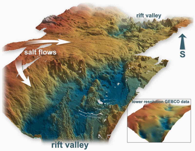
Bathymetry of a 70-kilometer long section of the rift zone in the Red Sea. In the lower right is the same section in the previous resolution. Credit: Graphics: N. Augustin, GEOMAR
The Red Sea has turned out to be an ideal study object for marine geologists. There they can observe the formation of an ocean in its early phase. However, the Red Sea seemed to go through a different birthing process than the other oceans. Now, scientists at the GEOMAR Helmholtz Centre for Ocean Research Kiel and the King Abdulaziz University in Jeddah have been able to show that salt glaciers have distorted the previous models. The study was just published in the international journal Earth and Planetary Science Letters.
Pacific, Atlantic and Indian Ocean, with the land masses of the Americas, Europe, Asia, Africa and Australia in between — that’s how we know our Earth. From a geologist’s point of view, however, this is only a snapshot. Over the course of Earth’s history, many different continents have formed and split again. In between oceans were created, new seafloor was formed and disappeared again: Plate tectonics is the generic term for these processes.
The Red Sea, where currently the Arabian Peninsula separates from Africa, is one of the few places on earth where the splitting of a continent and the emergence of the ocean can be observed. During a three-year joint project, the Jeddah Transect Project (JTP), researchers at the GEOMAR Helmholtz Centre for Ocean Research Kiel and the King Abdulaziz University (KAU) in Jeddah, Saudi Arabia, have taken a close look at this crack in Earth’s crust by means of seabed mapping, sampling and magnetic modeling. “The findings have shed new light on the early stages of oceanic basins, and they specifically change the school of thought on the Red Sea,” says Dr. Nico Augustin from GEOMAR, lead author of the study.
It is, and was, undisputed that a continent is stretched and thinned out by volcanic activity before it ruptures and a new ocean basin is formed. The rifting occurs where the greatest stretching takes place. However, the detailed processes during the break-up are debated in research. On the one hand, one needs to better understand the dynamics of our home planet. “On the other hand, most marine oil and gas resources are located near such former fracture zones. This research can therefore also have economic and political implications,” says Professor Colin Devey (GEOMAR), co-author of the study.
Until now, conventional knowledge said that a continent is breaking apart more or less simultaneously along an entire line, and the ocean basin is formed all at once. The Red Sea, however, did not fit into this picture. Here, a model was favored with several smaller fracture zones, lined up one after the other, that would unite gradually, which in turn would lead to a relatively slow emergence of the ocean during a long transition phase. “Our studies show that the Red Sea is not an exception but that it takes its place in line with the other ocean basins,” says Augustin. The previous picture we had of the ocean floor in the Red Sea was simply corrupted by salt glaciers. “The volcanic rocks we recovered are similar to those from other normal mid-ocean ridges,” says co-author Froukje van der Zwan, working on her PhD as part of the JTP.
During the early formation stages of the Red Sea, the area was covered by a very shallow sea that dried up repeatedly. This created thick salt deposits that later on broke apart with the continental crust. Over geologic time periods, salt shows tar-like behavior and begins to flow. “Our new high-resolution seabed maps and magnetic modeling show that the kilometer-thick salt deposits, after the break-up of the Arabian Plate from Africa, flowed like glaciers toward the newly created trench and thus over the oceanic crust due to gravity,” says Augustin. Since these submarine salt glaciers do not cover the rifting zone uniformly over the entire length, the impression of several small fracture zones was created.
The consequences of this discovery are profound: For one, there really seems to be only one single mechanism worldwide for the dispersal of a continent. And secondly, is not yet known how much ocean crust is covered by salt. This questions the previous dating of the opening of the Red Sea. In addition, the volcanically active trench rift zone of the Red Sea, surrounded by salt glaciers, is host of a giant sink filled with a very hot and very salty solution. “Since the sediment in the salt solution is rich in metals, this so-called Atlantis II Deep is also of economic interest,” says co-author Devey. It is quite conceivable that over the course of Earth’s history similar deposits associated with volcanism and salt deposits were created during the opening phase of other oceans. “Thus, our studies help to clarify older research questions. But they also provide starting points for new investigations in all of the oceans,” says Augustin.
Note : The above story is based on materials provided by Helmholtz Centre for Ocean Research Kiel (GEOMAR).
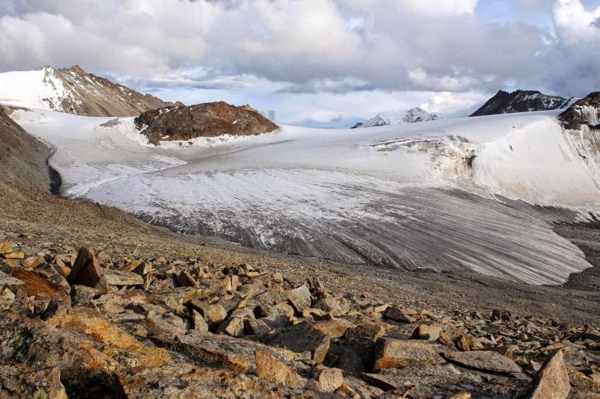
This image shows the Zhadang glacier south of lake Nam Tso on the nortern ridge of the Nyainqentanglha mountain range (Tibet, China). Credit: Tino Pieczonka (TU Dresden)
An international team led by glaciologists from the University of Colorado Boulder and Trent University in Ontario, Canada has completed the first mapping of virtually all of the world’s glaciers—including their locations and sizes—allowing for calculations of their volumes and ongoing contributions to global sea rise as the world warms.
The team mapped and catalogued some 198,000 glaciers around the world as part of the massive Randolph Glacier Inventory, or RGI, to better understand rising seas over the coming decades as anthropogenic greenhouse gases heat the planet. Led by CU-Boulder Professor Tad Pfeffer and Trent University Professor Graham Cogley, the team included 74 scientists from 18 countries, most working on an unpaid, volunteer basis.
The project was undertaken in large part to provide the best information possible for the recently released Fifth Assessment of the Intergovernmental Panel on Climate Change, or IPCC. While the Greenland and Antarctic ice sheets are both losing mass, it is the smaller glaciers that are contributing the most to rising seas now and that will continue to do so into the next century, said Pfeffer, a lead author on the new IPCC sea rise chapter and fellow at CU-Boulder’s Institute of Arctic and Alpine Research.
“I don’t think anyone could make meaningful progress on projecting glacier changes if the Randolph inventory was not available,” said Pfeffer, the first author on the RGI paper published online today in the Journal of Glaciology. Pfeffer said while funding for mountain glacier research has almost completely dried up in the United States in recent years with the exception of grants from NASA, there has been continuing funding by a number of European groups.
Since the world’s glaciers are expected to shrink drastically in the next century as the temperatures rise, the new RGI—named after one of the group’s meeting places in New Hampshire—is critical, said Pfeffer. In the RGI each individual glacier is represented by an accurate, computerized outline, making forecasts of glacier-climate interactions more precise.
“This means that people can now do research that they simply could not do before,” said Cogley, the corresponding author on the new Journal of Glaciology paper. “It’s now possible to conduct much more robust modeling for what might happen to these glaciers in the future.”
As part of the RGI effort, the team mapped intricate glacier complexes in places like Alaska, Patagonia, central Asia and the Himalayas, as well as the peripheral glaciers surrounding the two great ice sheets in Greenland and Antarctica, said Pfeffer. “In order to model these glaciers, we have to know their individual characteristics, not simply an average or aggregate picture. That was one of the most difficult parts of the project.”
The team used satellite images and maps to outline the area and location of each glacier. The researchers can combine that information with a digital elevation model, then use a technique known as “power law scaling” to determine volumes of various collections of glaciers.
In addition to impacting global sea rise, the melting of the world’s glaciers over the next 100 years will severely affect regional water resources for uses like irrigation and hydropower, said Pfeffer. The melting also has implications for natural hazards like “glacier outburst” floods that may occur as the glaciers shrink, he said.
The total extent of glaciers in the RGI is roughly 280,000 square miles or 727,000 square kilometers—an area slightly larger than Texas or about the size of Germany, Denmark and Poland combined. The team estimated that the corresponding total volume of sea rise collectively held by the glaciers is 14 to 18 inches, or 350 to 470 millimeters.
The new estimates are less than some previous estimates, and in total they are less than 1 percent of the amount of water stored in the Greenland and Antarctic ice sheets, which collectively contain slightly more than 200 feet, or 63 meters, of sea rise.
“A lot of people think that the contribution of glaciers to sea rise is insignificant when compared with the big ice sheets,” said Pfeffer, also a professor in CU-Boulder’s civil, environmental and architectural engineering department. “But in the first several decades of the present century it is going to be this glacier reservoir that will be the primary contributor to sea rise. The real concern for city planners and coastal engineers will be in the coming decades, because 2100 is pretty far off to have to make meaningful decisions.”
Part of the RGI was based on the Global Land Ice Measurements from Space Initiative, or GLIMS, which involved more than 60 institutions from around the world and which contributed the baseline dataset for the RGI. Another important research data tool for the RGI was the European-funded program “Ice2Sea,” which brings together scientific and operational expertise from 24 leading institutions across Europe and beyond.
The GLIMS glacier database and website are maintained by CU-Boulder’s National Snow and Ice Data Center, or NSIDC. The GLIMS research team at NSIDC includes principal investigator Richard Armstrong, technical lead Bruce Raup and remote-sensing specialist Siri Jodha Singh Khalsa.
NSIDC is part of the Cooperative Institute for Research in Environmental Sciences, or CIRES, a joint venture between CU-Boulder and the National Oceanic and Atmospheric Administration.
Note : The above story is based on materials provided by University of Colorado at Boulder
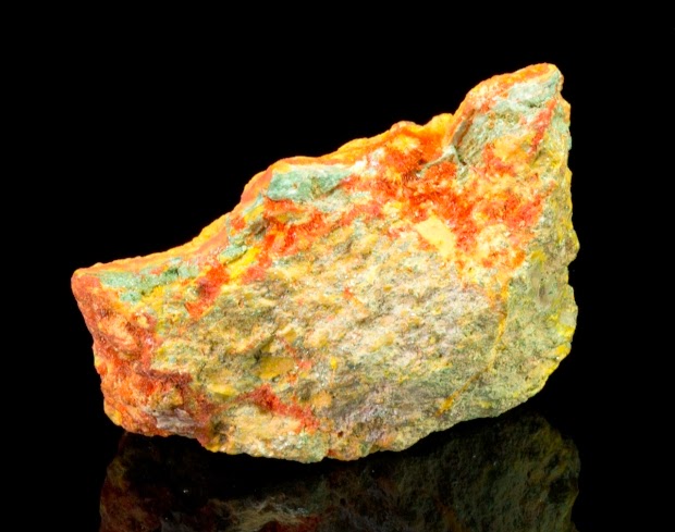
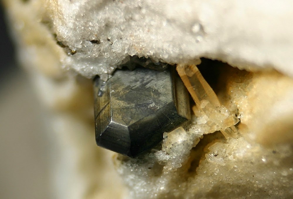
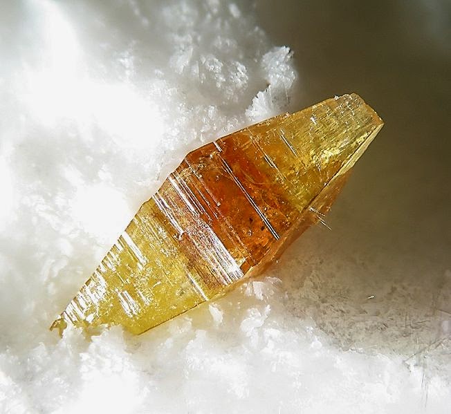
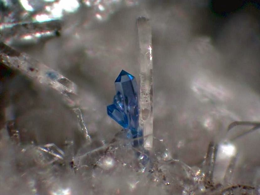
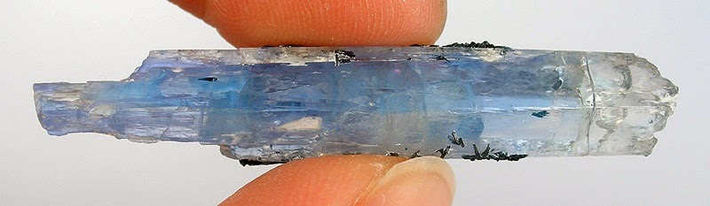
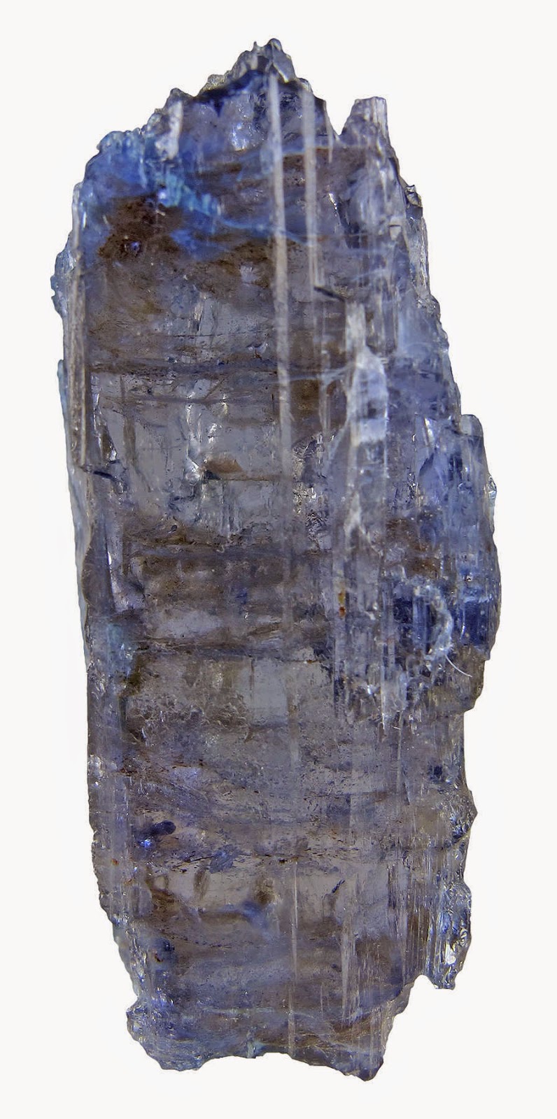
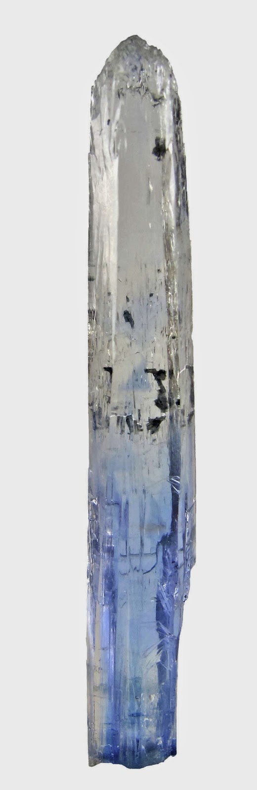
Chemical Formula: Al6(BO3)5(F,OH)3 Locality: Soktujberg, Adun-Tchilon and Baikal, Russia. Name Origin: Named after the Russian mineralogist, P. V. Jeremejev (1820-1899).
Jeremejevite is a rare aluminium borate mineral with variable fluoride and hydroxide ions. Its chemical formula is Al6(BO3)5(F,OH)3.
It was first described in 1883 for an occurrence on Mt. Soktui, Nerschinsk district, Adun-Chilon Mountains, Siberia. It was named after Russian mineralogist Pavel Vladimirovich Eremeev (Jeremejev, German) (1830–1899).
It occurs as a late hydrothermal phase in granitic pegmatites in association with albite, tourmaline, quartz and rarely gypsum. It has also been reported from the Pamir Mountains of Tajikistan, Namibia and the Eifel district, Germany.
Physical Properties
Cleavage: None Color: Colorless, White, Yellowish white, Bluish white. Density: 3.28 – 3.31, Average = 3.29 Diaphaneity: Transparent Fracture: Conchoidal – Fractures developed in brittle materials characterized by smoothly curving surfaces, (e.g. quartz). Hardness: 7 – Quartz Luminescence: Non-fluorescent. Luster: Vitreous (Glassy) Streak: white
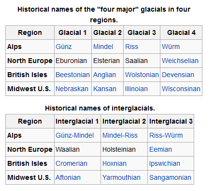
The Holocene is a geological epoch which began at the end of the Pleistocene (at 11,700 calendar years BP) and continues to the present. The Holocene is part of the Quaternary period. Its name comes from the Greek words ὅλος (holos, whole or entire) and καινός (kainos, new), meaning “entirely recent”. It has been identified with the current warm period, known as MIS 1 and based on that past evidence, can be considered an interglacial in the current ice age.
The Holocene also encompasses within it the growth and impacts of the human species world-wide, including all its written history and overall significant transition toward urban living in the present. Human impacts of the modern era on the Earth and its ecosystems may be considered of global significance for future evolution of living species, including approximately synchronous lithospheric evidence, or more recently atmospheric evidence of human impacts. Given these, a new term Anthropocene, is specifically proposed and used informally only for the very latest part of modern history and of significant human impact since the epoch of the Neolithic Revolution (around 12,000 years BP).
Overview
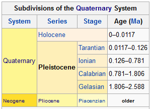
It is accepted by the International Commission on Stratigraphy that the Holocene started approximately 11,700 years BP (before present). The period follows the last glacial period (regionally known as the Wisconsinan Glacial Period, the Baltic-Scandinavian Ice Age, or the Weichsel glacial). The Holocene can be subdivided into five time intervals, or chronozones, based on climatic fluctuations:
Preboreal (10 ka – 9 ka),
Boreal (9 ka – 8 ka),
Atlantic (8 ka – 5 ka),
Subboreal (5 ka – 2.5 ka) and
Subatlantic (2.5 ka – present).
Note: “ka” means “thousand years” (non-calibrated C14 dates)
The Blytt-Sernander classification of climatic periods defined, initially, by plant remains in peat mosses, is now being explored currently by geologists working in different regions studying sea levels, peat bogs and ice core samples by a variety of methods, with a view toward further verifying and refining the Blytt-Sernander sequence. They find a general correspondence across Eurasia and North America, though the method was once thought to be of no interest. The scheme was defined for Northern Europe, but the climate changes were claimed to occur more widely. The periods of the scheme include a few of the final pre-Holocene oscillations of the last glacial period and then classify climates of more recent prehistory.
Paleontologists have defined no faunal stages for the Holocene. If subdivision is necessary, periods of human technological development, such as the Mesolithic, Neolithic, and Bronze Age, are usually used. However, the time periods referenced by these terms vary with the emergence of those technologies in different parts of the world.
Climatically, the Holocene may be divided evenly into the Hypsithermal and Neoglacial periods; the boundary coincides with the start of the Bronze Age in European civilization. According to some scholars, a third division, the Anthropocene, began in the 18th century.
Continental motions due to plate tectonics are less than a kilometre over a span of only 10,000 years. However, ice melt caused world sea levels to rise about 35 m (115 ft) in the early part of the Holocene. In addition, many areas above about 40 degrees north latitude had been depressed by the weight of the Pleistocene glaciers and rose as much as 180 m (590 ft) due to post-glacial rebound over the late Pleistocene and Holocene, and are still rising today.
The sea level rise and temporary land depression allowed temporary marine incursions into areas that are now far from the sea. Holocene marine fossils are known from Vermont, Quebec, Ontario, Maine, New Hampshire, and Michigan. Other than higher-latitude temporary marine incursions associated with glacial depression, Holocene fossils are found primarily in lakebed, floodplain, and cave deposits. Holocene marine deposits along low-latitude coastlines are rare because the rise in sea levels during the period exceeds any likely tectonic uplift of non-glacial origin.
Post-glacial rebound in the Scandinavia region resulted in the formation of the Baltic Sea. The region continues to rise, still causing weak earthquakes across Northern Europe. The equivalent event in North America was the rebound of Hudson Bay, as it shrank from its larger, immediate post-glacial Tyrrell Sea phase, to near its present boundaries.
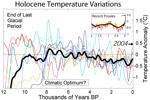
Climate
Temperature variations during the Holocene
Climate has been fairly stable over the Holocene. Ice core records show that before the Holocene there was global warming after the end of the last ice age and cooling periods, but climate changes became more regional at the start of the Younger Dryas. During the transition from last glacial to holocene, the Huelmo/Mascardi Cold Reversal in the Southern Hemisphere began before the Younger Dryas, and the maximum warmth flowed south to north from 11,000 to 7,000 years ago. It appears that this was influenced by the residual glacial ice remaining in the Northern Hemisphere until the later date.
The hypsithermal was a period of warming in which the global climate became warmer. However, the warming was probably not uniform across the world. This period of warmth ended about 5,500 years ago with the descent into the Neoglacial. At that time, the climate was not unlike today’s, but there was a slightly warmer period from the 10th–14th centuries known as the Medieval Warm Period. This was followed by the Little Ice Age, from the 13th or 14th century to the mid 19th century, which was a period of significant cooling, though not everywhere as severe as previous times during neoglaciation.
The Holocene warming is an interglacial period and there is no reason to believe that it represents a permanent end to the current ice age. However, the current global warming may result in the Earth becoming warmer than the Eemian Stage, which peaked at roughly 125,000 years ago and was warmer than the Holocene. This prediction is sometimes referred to as a super-interglacial.
Compared to glacial conditions, habitable zones have expanded northwards, reaching their northernmost point during the hypsithermal. Greater moisture in the polar regions has caused the disappearance of steppe-tundra.
Animal and plant life have not evolved much during the relatively short Holocene, but there have been major shifts in the distributions of plants and animals. A number of large animals including mammoths and mastodons, saber-toothed cats like Smilodon and Homotherium, and giant sloths disappeared in the late Pleistocene and early Holocene—especially in North America, where animals that survived elsewhere (including horses and camels) became extinct. This extinction of American megafauna has been explained as caused by the arrival of the ancestors of Amerindians; though most scientists assert that climatic change also contributed. In addition, a discredited bolide impact over North America which was hypothesized to have triggered the Younger Dryas.
Throughout the world, ecosystems in cooler climates that were previously regional have been isolated in higher altitude ecological “islands”.
The 8.2 ka event, an abrupt cold spell recorded as a negative excursion in the δ18O record lasting 400 years, is the most prominent climatic event occurring in the Holocene epoch, and may have marked a resurgence of ice cover. It is thought that this event was caused by the final drainage of Lake Agassiz, which had been confined by the glaciers, disrupting the thermohaline circulation of the Atlantic.
Human developments
The beginning of the Holocene corresponds with the beginning of the Mesolithic age in most of Europe; but in regions such as the Middle East and Anatolia with a very early neolithisation, Epipaleolithic is preferred in place of Mesolithic. Cultures in this period include: Hamburgian, Federmesser, and the Natufian culture, during which the oldest inhabited places still existing on Earth were first settled, such as Jericho in the Middle East, as well as evolving archeological evidence of proto-religion at locations such as Göbekli Tepe, as long ago as the 9th millennium BC.
Both are followed by the aceramic Neolithic (Pre-Pottery Neolithic A and Pre-Pottery Neolithic B) and the pottery Neolithic. The Late Holocene brought advancements such as the bow and arrow and saw new methods of warfare in North America. Spear throwers and their large points were replaced by the bow and arrow with its small narrow points beginning in Oregon and Washington. Villages built on defensive bluffs indicate increased warfare, leading to food gathering in communal groups rather than individual hunting for protection.
Impact events
Many meteorite events which occurred in the Holocene have so far been found in Europe, in bodies of water such as the Indian Ocean and in Russia, near the remote region of Siberia. Siberia is also the site of a modern impact event in 1908 known as the Tunguska Event. It has been speculated that an impact such as that represented today by the Burckle Crater could have dramatically affected human culture in its early history by the creation of megatsunamis, perhaps inspiring deluge or inundation myths such as that of Noah’s Flood.
Note : The above story is based on materials provided by Wikipedia
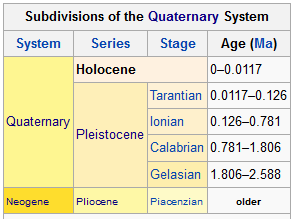
The Pleistocene is the geological epoch which lasted from about 2,588,000 to 11,700 years ago, spanning the world’s recent period of repeated glaciations.
Charles Lyell introduced this term in 1839 to describe strata in Sicily that had at least 70% of their molluscan fauna still living today. This distinguished it from the older Pliocene Epoch, which Lyell had originally thought to be the youngest fossil rock layer. He constructed the name “Pleistocene” (“Most New” or “Newest”) from the Greek πλεῖστος, pleīstos, “most”, and καινός, kainós (latinized as cænus), “new”; this contrasting with the immediately preceding Pleiocene (“More New” or “Newer”, from πλείων, pleíōn, “more”, and kainós; usual spelling: Pliocene), and the immediately subsequent Holocene (“wholly new” or “entirely new”, from ὅλος, hólos, “whole”, and kainós) epoch, which extends to the present time.
The Pleistocene is the first epoch of the Quaternary Period or sixth epoch of the Cenozoic Era. The end of the Pleistocene corresponds with the end of the last glacial period. It also corresponds with the end of the Paleolithic age used in archaeology. In the ICS timescale, the Pleistocene is divided into four stages or ages, the Gelasian, Calabrian, Ionian and Tarantian. All of these stages were defined in southern Europe. In addition to this international subdivision, various regional subdivisions are often used.
Before a change finally confirmed in 2009 by the International Union of Geological Sciences, the time boundary between the Pleistocene and the preceding Pliocene was regarded as being at 1.806 million years before the present, as opposed to the currently accepted 2.588 million years BP: publications from the preceding years may use either definition of the period.
Dating
The Pleistocene has been dated from 2.588 million (±5,000) to 11,700 years before present (BP), with the end date expressed in radiocarbon years as 10,000 carbon-14 years BP. It covers most of the latest period of repeated glaciation, up to and including the Younger Dryas cold spell. The end of the Younger Dryas has been dated to about 9640 BC (11,654 calendar years BP). It was not until after the development of radiocarbon dating, however, that Pleistocene archaeological excavations shifted to stratified caves and rock-shelters as opposed to open-air river-terrace sites.
In 2009 the International Union of Geological Sciences (IUGS) confirmed a change in time period for the Pleistocene, changing the start date from 1.806 to 2.588 million years BP, and accepted the base of the Gelasian as the base of the Pleistocene, namely the base of the Monte San Nicola GSSP.The IUGS has yet to approve a type section, Global Boundary Stratotype Section and Point (GSSP), for the upper Pleistocene/Holocene boundary (i.e. the upper boundary). The proposed section is the North Greenland Ice Core Project ice core 75° 06′ N 42° 18′ W. The lower boundary of the Pleistocene Series is formally defined magnetostratigraphically as the base of the Matuyama (C2r) chronozone, isotopic stage 103. Above this point there are notable extinctions of the calcareous nanofossils: Discoaster pentaradiatus and Discoaster surculus.
The Pleistocene covers the recent period of repeated glaciations. The name Plio-Pleistocene has in the past been used to mean the last ice age. The revised definition of the Quaternary, by pushing back the start date of the Pleistocene to 2.58 Ma, results in the inclusion of all the recent repeated glaciations within the Pleistocene.
Paleogeography and climate
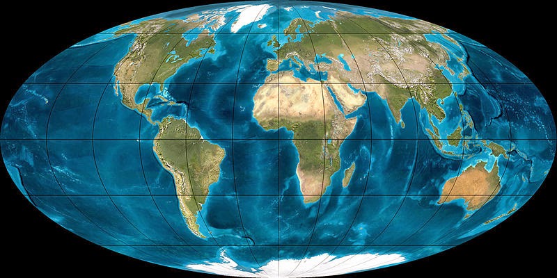
The modern continents were essentially at their present positions during the Pleistocene, the plates upon which they sit probably having moved no more than 100 km relative to each other since the beginning of the period.
According to Mark Lynas (through collected data), the Pleistocene’s overall climate could be characterized as a continuous El Niño with trade winds in the south Pacific weakening or heading east, warm air rising near Peru, warm water spreading from the west Pacific and the Indian Ocean to the east Pacific, and other El Niño markers.
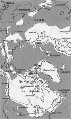
Glacial features
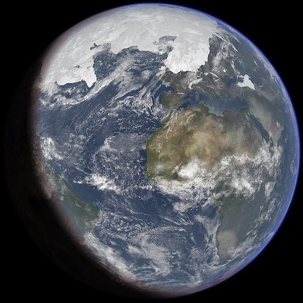
Pleistocene climate was marked by repeated glacial cycles in which continental glaciers pushed to the 40th parallel in some places. It is estimated that, at maximum glacial extent, 30% of the Earth’s surface was covered by ice. In addition, a zone of permafrost stretched southward from the edge of the glacial sheet, a few hundred kilometres in North America, and several hundred in Eurasia. The mean annual temperature at the edge of the ice was −6 °C (21 °F); at the edge of the permafrost, 0 °C (32 °F).
The maximum extent of glacial ice in the north polar area during the Pleistocene period.
Each glacial advance tied up huge volumes of water in continental ice sheets 1,500 to 3,000 metres (4,900–9,800 ft) thick, resulting in temporary sea-level drops of 100 metres (300 ft) or more over the entire surface of the Earth. During interglacial times, such as at present, drowned coastlines were common, mitigated by isostatic or other emergent motion of some regions.
The effects of glaciation were global. Antarctica was ice-bound throughout the Pleistocene as well as the preceding Pliocene. The Andes were covered in the south by the Patagonian ice cap. There were glaciers in New Zealand and Tasmania. The current decaying glaciers of Mount Kenya, Mount Kilimanjaro, and the Ruwenzori Range in east and central Africa were larger. Glaciers existed in the mountains of Ethiopia and to the west in the Atlas mountains.
In the northern hemisphere, many glaciers fused into one. The Cordilleran ice sheet covered the North American northwest; the east was covered by the Laurentide. The Fenno-Scandian ice sheet rested on northern Europe, including Great Britain; the Alpine ice sheet on the Alps. Scattered domes stretched across Siberia and the Arctic shelf. The northern seas were ice-covered.
South of the ice sheets large lakes accumulated because outlets were blocked and the cooler air slowed evaporation. When the Laurentide ice sheet retreated, north central North America was totally covered by Lake Agassiz. Over a hundred basins, now dry or nearly so, were overflowing in the North American west. Lake Bonneville, for example, stood where Great Salt Lake now does. In Eurasia, large lakes developed as a result of the runoff from the glaciers. Rivers were larger, had a more copious flow, and were braided. African lakes were fuller, apparently from decreased evaporation. Deserts on the other hand were drier and more extensive. Rainfall was lower because of the decrease in oceanic and other evaporation.
Major events
Over 11 major glacial events have been identified, as well as many minor glacial events. A major glacial event is a general glacial excursion, termed a “glacial.” Glacials are separated by “interglacials”. During a glacial, the glacier experiences minor advances and retreats. The minor excursion is a “stadial”; times between stadials are “interstadials”.
These events are defined differently in different regions of the glacial range, which have their own glacial history depending on latitude, terrain and climate. There is a general correspondence between glacials in different regions. Investigators often interchange the names if the glacial geology of a region is in the process of being defined. However, it is generally incorrect to apply the name of a glacial in one region to another.
For most of the 20th century only a few regions had been studied and the names were relatively few. Today the geologists of different nations are taking more of an interest in Pleistocene glaciology. As a consequence, the number of names is expanding rapidly and will continue to expand. Many of the advances and stadials remain unnamed. Also, the terrestrial evidence for some of them has been erased or obscured by larger ones, but evidence remains from the study of cyclical climate changes.
The glacials in the following tables show historical usages, are a simplification of a much more complex cycle of variation in climate and terrain, and are generally no longer used. These names have been abandoned in favor of numeric data because many of the correlations were found to be either inexact or incorrect and more than four major glacials have been recognized since the historical terminology was established.
Corresponding to the terms glacial and interglacial, the terms pluvial and interpluvial are in use (Latin: pluvia, rain). A pluvial is a warmer period of increased rainfall; an interpluvial, of decreased rainfall. Formerly a pluvial was thought to correspond to a glacial in regions not iced, and in some cases it does. Rainfall is cyclical also. Pluvials and interpluvials are widespread.
There is no systematic correspondence of pluvials to glacials, however. Moreover, regional pluvials do not correspond to each other globally. For example, some have used the term “Riss pluvial” in Egyptian contexts. Any coincidence is an accident of regional factors. Only a few of the names for pluvials in restricted regions have been strategraphically defined.
Palaeocycles
The sum of transient factors acting at the Earth’s surface is cyclical: climate, ocean currents and other movements, wind currents, temperature, etc. The waveform response comes from the underlying cyclical motions of the planet, which eventually drag all the transients into harmony with them. The repeated glaciations of the Pleistocene were caused by the same factors.
Milankovitch cycles
Glaciation in the Pleistocene was a series of glacials and interglacials, stadials and interstadials, mirroring periodic changes in climate. The main factor at work in climate cycling is now believed to be Milankovitch cycles. These are periodic variations in regional and planetary solar radiation reaching the Earth caused by several repeating changes in the Earth’s motion.
Milankovitch cycles cannot be the sole factor responsible for the variations in climate since they explain neither the long term cooling trend over the Plio-Pleistocene, nor the millennial variations in the Greenland Ice Cores. Milankovitch pacing seems to best explain glaciation events with periodicity of 100,000, 40,000, and 20,000 years. Such a pattern seems to fit the information on climate change found in oxygen isotope cores. The timing of our present interglacial interval (known as the Holocene, Postglacial, or the Present Interglacial) to that of the previous interglacial, beginning about 130,000 years ago (The Eemian Interglacial), suggests that the next glacial would likely begin in about 3,000 years.
Oxygen isotope ratio cycles
In oxygen isotope ratio analysis, variations in the ratio of O18 to O16 (two isotopes of oxygen) by mass (measured by a mass spectrometer) present in the calcite of oceanic core samples is used as a diagnostic of ancient ocean temperature change and therefore of climate change. Cold oceans are richer in O18, which is included in the tests of the microorganisms (foraminifera) contributing the calcite.
A more recent version of the sampling process makes use of modern glacial ice cores. Although less rich in O18 than sea water, the snow that fell on the glacier year by year nevertheless contained O18 and O16 in a ratio that depended on the mean annual temperature.
Temperature and climate change are cyclical when plotted on a graph of temperature versus time. Temperature coordinates are given in the form of a deviation from today’s annual mean temperature, taken as zero. This sort of graph is based on another of isotope ratio versus time. Ratios are converted to a percentage difference from the ratio found in standard mean ocean water (SMOW).
The graph in either form appears as a waveform with overtones. One half of a period is a Marine isotopic stage (MIS). It indicates a glacial (below zero) or an interglacial (above zero). Overtones are stadials or interstadials.
According to this evidence, Earth experienced 102 MIS stages beginning at about 2.588 Ma BP in the Early Pleistocene Gelasian. Early Pleistocene stages were shallow and frequent. The latest were the most intense and most widely spaced.
By convention, stages are numbered from the Holocene, which is MIS1. Glacials receive an even number; interglacials, odd. The first major glacial was MIS2-4 at about 85–11 ka BP. The largest glacials were 2, 6, 12, and 16; the warmest interglacials, 1, 5, 9 and 11. For matching of MIS numbers to named stages, see under the articles for those names.
Fauna
Both marine and continental faunas were essentially modern and many animals, specifically, mammals were much larger than their modern relatives .
The severe climatic changes during the ice age had major impacts on the fauna and flora. With each advance of the ice, large areas of the continents became totally depopulated, and plants and animals retreating southward in front of the advancing glacier faced tremendous stress. The most severe stress resulted from drastic climatic changes, reduced living space, and curtailed food supply. A major extinction event of large mammals (megafauna), which included mammoths, mastodons, saber-toothed cats, glyptodons, ground sloths, Irish elk, cave bears, and short-faced bears, began late in the Pleistocene and continued into the Holocene. Neanderthals also became extinct during this period. At the end of the last ice age, cold-blooded animals, smaller mammals like wood mice, migratory birds, and swifter animals like whitetail deer had replaced the megafauna and migrated north.
The extinctions were especially severe in North America where native horses and camels were eliminated.
Asian land mammal ages (ALMA) include Zhoukoudianian, Nihewanian, and Yushean.
European land mammal ages (ELMA) include Gelasian (2.5—1.8 Ma).
North American land mammal ages (NALMA) include Blancan (4.75–1.8), Irvingtonian (1.8–0.24) and Rancholabrean (0.24–0.01) in millions of years. The Blancan extends significantly back into the Pliocene.
South American land mammal ages (SALMA) include Uquian (2.5–1.5), Ensenadan (1.5–0.3) and Lujanian (0.3–0.01) in millions of years. The Uquian extends significantly back into the Pliocene.
Humans
Scientific evidence indicates that humans evolved into their present form during the Pleistocene.In the beginning of the Pleistocene Paranthropus species are still present, as well as early human ancestors, but during the lower Palaeolithic they disappeared, and the only hominid species found in fossilic records is Homo erectus for much of the Pleistocene. The Middle and late Palaeolithic saw the appearance of new types of humans, as well as the development of more elaborate tools than found in previous eras. According to mitochondrial timing techniques, modern humans migrated from Africa after the Riss glaciation in the middle Palaeolithic during the Eemian Stage, spreading all over the ice-free world during the late Pleistocene. A 2005 study posits that humans in this migration interbred with archaic human forms already outside of Africa by the late Pleistocene, incorporating archaic human genetic material into the modern human gene pool.
Deposits
Pleistocene non-marine sediments are found primarily in fluvial deposits, lakebeds, slope and loess deposits as well as in the large amounts of material moved about by glaciers. Less common are cave deposits, travertines and volcanic deposits (lavas, ashes). Pleistocene marine deposits are found primarily in shallow marine basins mostly (but with important exceptions) in areas within a few tens of kilometers of the modern shoreline. In a few geologically active areas such as the Southern California coast, Pleistocene marine deposits may be found at elevations of several hundred meters.
Note : The above story is based on materials provided by Wikipedia
The Quaternary Period /kwəˈtɜrnəri/ is the most recent of the three periods of the Cenozoic Era in the geologic time scale of the ICS.It follows the Neogene Period and spans from 2.588 ± 0.005 million years ago to the present. Traditionally it was preceded by Tertiary which is no longer recognized as a formal geological unit but is still in colloquial use.
This relatively short geological period is characterized by a series of glaciations and by the appearance and expansion of anatomically modern humans.
Also of note, all objects that are suitable for carbon dating are enclosed in this period.
The Quaternary includes two geologic epochs: the Pleistocene and Holocene.
A proposed but as yet informal third epoch, the Anthropocene, has also gained credence as the time in which humans began to profoundly affect and change the global environment, although its start date is still disputed.
Research history
The term Quaternary (“fourth”) was proposed by Giovanni Arduino in 1759 for alluvial deposits in the Po River valley in northern Italy. It was introduced by Jules Desnoyers in 1829 for sediments of France’s Seine Basin that seemed clearly to be younger than Tertiary Period rocks.
The Quaternary Period follows the Neogene Period and extends to the present. The Quaternary covers the time span of glaciations classified as the Pleistocene, and includes the present interglacial period, the Holocene.
This places the start of the Quaternary at the onset of Northern Hemisphere glaciation approximately 2.6 million years ago. Prior to 2009, the Pleistocene was defined to be from 1.805 million years ago to the present, so the current definition of the Pleistocene includes a portion of what was, prior to 2009, defined as the Pliocene.
Quaternary stratigraphers usually worked with regional subdivisions. From the 1970s, the International Commission on Stratigraphy (ICS) tried to make a single geologic time scale based on GSSP’s, which could be used internationally. The Quaternary subdivisions were defined based on biostratigraphy instead of paleoclimate.
This led to the problem that the proposed base of the Pleistocene was at 1.805 Mya, long after the start of the major glaciations of the northern hemisphere. The ICS then proposed to abolish use of the name Quaternary altogether, which appeared unacceptable to the International Union for Quaternary Research (INQUA).
In 2009, it was decided to make the Quaternary the youngest period of the Cenozoic Era with its base at 2.588 Mya and including the Gelasian stage, which was formerly considered part of the Neogene Period and Pliocene Epoch.
Geology
The 2.6 million years of the Quaternary represents the time during which recognizable humans existed. Over this short time period, there has been relatively little change in the distribution of the continents due to plate tectonics.
The Quaternary geological record is preserved in greater detail than that for earlier periods.
The major geographical changes during this time period included the emergence of the Strait of Bosphorus and Skagerrak during glacial epochs, which respectively turned the Black Sea and Baltic Sea into fresh water, followed by their flooding (and return to salt water) by rising sea level; the periodic filling of the English Channel, forming a land bridge between Britain and the European mainland; the periodic closing of the Bering Strait, forming the land bridge between Asia and North America; and the periodic flash flooding of Scablands of the American Northwest by glacial water.
The current extent of Hudson Bay, the Great Lakes and other major lakes of North America are a consequence of the Canadian Shield’s readjustment since the last ice age; different shorelines have existed over the course of Quaternary time.
Climate
The climate was one of periodic glaciations with continental glaciers moving as far from the poles as 40 degrees latitude. There was a major extinction of large mammals in Northern areas at the end of the Pleistocene Epoch. Many forms such as saber-toothed cats, mammoths, mastodons, glyptodonts, etc., became extinct worldwide. Others, including horses, camels and American cheetahs became extinct in North America.
Quaternary glaciation
Glaciation took place repeatedly during the Quaternary Ice Age – a term coined by Schimper in 1839 that began with the start of the Quaternary about 2.58 Mya and continues to the present-day.
Last glacial period
Artist’s impression of Earth during the Last Glacial Maximum
In 1821, a Swiss engineer, Ignaz Venetz, presented an article in which he suggested the presence of traces of the passage of a glacier at a considerable distance from the Alps. This idea was initially disputed by another Swiss scientist, Louis Agassiz, but when he undertook to disprove it, he ended up affirming his colleague’s hypothesis. A year later, Agassiz raised the hypothesis of a great glacial period that would have had long-reaching general effects. This idea gained him international fame and led to the establishment of the Glacial Theory.
In time, thanks to the refinement of geology, it has been demonstrated that there were several periods of glacial advance and retreat and that past temperatures on Earth were very different from today. In particular, the Milankovitch cycles of Milutin Milankovitch are based on the premise that variations in incoming solar radiation are a fundamental factor controlling Earth’s climate.
During this time, substantial glaciers advanced and retreated over much of North America and Europe, parts of South America and Asia, and all of Antarctica. The Great Lakes formed and giant mammals thrived in parts of North America and Eurasia not covered in ice. These mammals became extinct when the glacial period Age ended about 11,700 years ago. Modern humans evolved about 190,000 years ago (source: Leakey). During the Quaternary period, mammals, flowering plants, and insects dominated the land.
Note : The above story is based on materials provided by Wikipedia
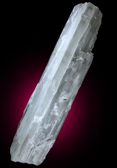
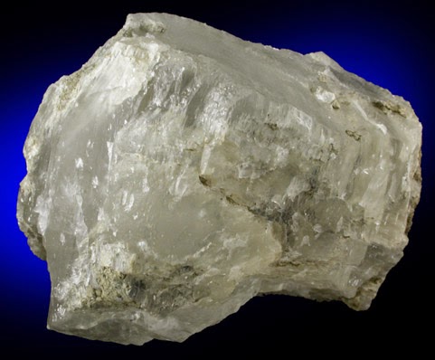
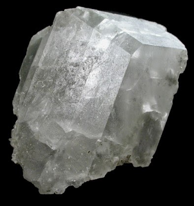
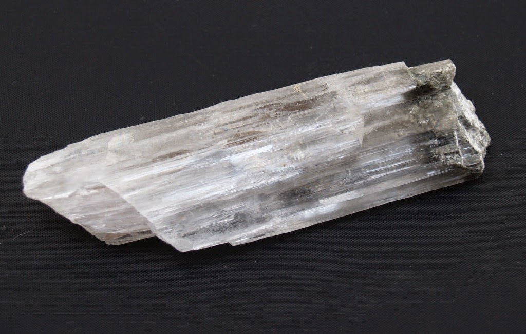
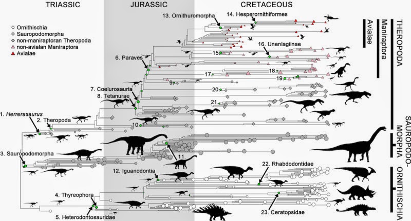
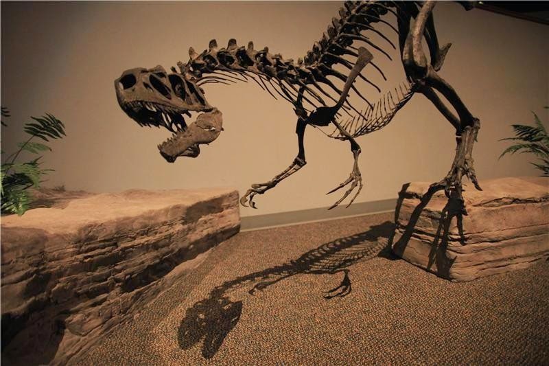
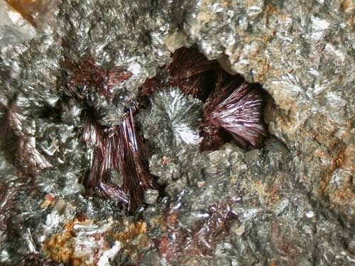 Chemical Formula: Sb2S2O