Using friction experiments University of Liverpool scientists have shown that frictional melting plays a role in determining how a volcano will erupt. Credit: Dr. Jackie Kendrick
A new discovery in the study of how lava dome volcanoes erupt may help in the development of methods to predict how a volcanic eruption will behave, say scientists at the University of Liverpool.
Volcanologists at the University have discovered that a process called frictional melting plays a role in determining how a volcano will erupt, by dictating how fast magma can ascend to the surface, and how much resistance it faces en-route.
The process occurs in lava dome volcanoes when magma and rocks melt as they rub against each other due to intense heat. This creates a stop start movement in the magma as it makes its way towards Earth’s surface. The magma sticks to the rock and stops moving until enough pressure builds up, prompting it to shift forward again (a process called stick-slip).
Volcanologist, Dr Jackie Kendrick, who lead the research said: “Seismologists have long known that frictional melting takes place when large tectonic earthquakes occur. It is also thought that the stick-slip process that frictional melting generates is concurrent to ‘seismic drumbeats’ which are the regular, rhythmic small earthquakes which have been recently found to accompany large volcanic eruptions.
“Using friction experiments we have shown that the extent of frictional melting depends on the composition of the rock and magma, which determines how fast or slow the magma travels to the surface during the eruption.”
Analysis of lava collected from Mount St. Helens, USA and the Soufrière Hills volcano in Montserrat by volcanology researchers from the University’s School of Environmental Sciences revealed remnants of pseudotachylyte, a cooled frictional melt. Evidence showed that the process took place in the conduit, the channel which lava passes through on its way to erupt.
Dr Kendrick, from the University’s School of Environmental Sciences, added: “The closer we get to understanding the way magma behaves, the closer we will get to the ultimate goal: predicting volcanic activity when unrest begins. Whilst we can reasonably predict when a volcanic eruption is about to happen, this new knowledge will help us to predict how the eruption will behave.
“With a rapidly growing population inhabiting the flanks of active volcanoes, understanding the behaviour of lava domes becomes an increasing challenge for volcanologists.”
Note : The above story is based on materials provided by University of Liverpool.
Jarosite Bristol Silver Mine, Pioche, Lincoln County, Nevada, USA Miniature, 5.8 x 5.7 x 4.5 cm “Courtesy of Rob Lavinsky, The Arkenstone, www.iRocks.com”
Chemical Formula: KFe3+3(SO4)2(OH)6 Locality: Barranco Jaroso in southern Spain. Name Origin: Named after its locality.
Jarosite is a basic hydrous sulfate of potassium and iron with a chemical formula of KFe3+3(SO4)2(OH)6. This sulfate mineral is formed in ore deposits by the oxidation of iron sulfides. Jarosite is often produced as a byproduct during the purification and refining of zinc and is also commonly associated with acid mine drainage and acid sulfate soil environments.
History
Jarosite was first described in 1852 by August Breithaupt in the Barranco del Jaroso in the Sierra Almagrera (near Los Lobos, Cuevas del Almanzora, Almería, Spain). The name jarosite is also directly derived from Jara, the Spanish name of a yellow flower that belongs to the genus cistus and grows in this sierra. The mineral and the flower have the same color.
In 2004 jarosite was detected on Mars by a Mössbauer spectrometer on the MER-B rover, which has been interpreted as strong evidence that Mars once possessed large amounts of liquid water.
Mysterious spheres of clay, 1.5 to 5 inches in diameter, covered with jarosite have recently been discovered beneath the Temple of the Feathered Serpent an ancient six level stepped pyramid 30 miles from Mexico City.
The Pliocene is the period in the geologic timescale that extends from 5.332 million to 2.588 million years before present. It is the second and youngest epoch of the Neogene Period in the Cenozoic Era. The Pliocene follows the Miocene Epoch and is followed by the Pleistocene Epoch. Prior to the 2009 revision of the geologic time scale, which placed the 4 most recent major glaciations entirely within the Pleistocene, the Pliocene also included the Gelasian stage, which lasted from 2.588 to 1.806 million years ago, and is now included in the Pleistocene.
As with other older geologic periods, the geological strata that define the start and end are well identified but the exact dates of the start and end of the epoch are slightly uncertain. The boundaries defining the Pliocene are not set at an easily identified worldwide event but rather at regional boundaries between the warmer Miocene and the relatively cooler Pleistocene. The upper boundary was set at the start of the Pleistocene glaciations.
Etymology
The Pliocene was named by Sir Charles Lyell. The name comes from the Greek words πλεῖον (pleion, “more”) and καινός (kainos, “new”) and means roughly “continuation of the recent”, referring to the essentially modern marine mollusc faunas. H.W. Fowler called the term (along with other examples such as pleistocene and miocene) a “regrettable barbarism” and an indication that even “a good classical scholar” such as Lyell should have requested a philologist’s help when coining words.
Subdivisions
In the official timescale of the ICS, the Pliocene is subdivided into two stages. From youngest to oldest they are:
Piacenzian (3.600–2.588 Ma)
Zanclean (5.332–3.600 Ma)
The Piacenzian is sometimes referred to as the Late Pliocene, whereas the Zanclean is referred to as the Early Pliocene.In the system of
North American Land Mammal Ages (NALMA) include Hemphillian (9–4.75 Ma), and Blancan (4.75–1.806 Ma). The Blancan extends forward into the Pleistocene.
South American Land Mammal Ages (SALMA) include Montehermosan (6.8–4.0 Ma), Chapadmalalan (4.0–3.0 Ma) and Uquian (3.0–1.2 Ma).
In the Paratethys area (central Europe and parts of western Asia) the Pliocene contains the Dacian (roughly equal to the Zanclean) and Romanian (roughly equal to the Piacenzian and Gelasian together) stages. As usual in stratigraphy, there are many other regional and local subdivisions in use.In Britain the Pliocene is divided into the following stages (old to young): Gedgravian, Waltonian, Pre-Ludhamian, Ludhamian, Thurnian, Bramertonian or Antian, Pre-Pastonian or Baventian, Pastonian and Beestonian. In the Netherlands the Pliocene is divided into these stages (old to young): Brunssumian C, Reuverian A, Reuverian B, Reuverian C, Praetiglian, Tiglian A, Tiglian B, Tiglian C1-4b, Tiglian C4c, Tiglian C5, Tiglian C6 and Eburonian. The exact correlations between these local stages and the ICS stages is still a matter of detail.
Climate
Mid-Pliocene reconstructed annual sea surface temperature anomaly
The global average temperature in the mid-Pliocene (3.3–3 mya) was 2–3 °C higher than today,global sea level 25 m higher and the Northern hemisphere ice sheet was ephemeral before the onset of extensive glaciation over Greenland that occurred in the late Pliocene around 3 Ma. The formation of an Arctic ice cap is signaled by an abrupt shift in oxygen isotope ratios and ice-rafted cobbles in the North Atlantic and North Pacific ocean beds. Mid-latitude glaciation was probably underway before the end of the epoch. The global cooling that occurred during the Pliocene may have spurred on the disappearance of forests and the spread of grasslands and savannas.
Paleogeography
Continents continued to drift, moving from positions possibly as far as 250 km from their present locations to positions only 70 km from their current locations. South America became linked to North America through the Isthmus of Panama during the Pliocene, making possible the Great American Interchange and bringing a nearly complete end to South America’s distinctive large marsupial predator and native ungulate faunas. The formation of the Isthmus had major consequences on global temperatures, since warm equatorial ocean currents were cut off and an Atlantic cooling cycle began, with cold Arctic and Antarctic waters dropping temperatures in the now-isolated Atlantic Ocean.
Africa’s collision with Europe formed the Mediterranean Sea, cutting off the remnants of the Tethys Ocean. The border between the Miocene and the Pliocene is also the time of the Messinian salinity crisis.
Sea level changes exposed the land-bridge between Alaska and Asia.
Pliocene marine rocks are well exposed in the Mediterranean, India, and China. Elsewhere, they are exposed largely near shores.
Flora
The change to a cooler, dry, seasonal climate had considerable impacts on Pliocene vegetation, reducing tropical species worldwide. Deciduous forests proliferated, coniferous forests and tundra covered much of the north, and grasslands spread on all continents (except Antarctica). Tropical forests were limited to a tight band around the equator, and in addition to dry savannahs, deserts appeared in Asia and Africa.
Fauna
Both marine and continental faunas were essentially modern, although continental faunas were a bit more primitive than today. The first recognizable hominins, the australopithecines, appeared in the Pliocene.
The land mass collisions meant great migration and mixing of previously isolated species, such as in the Great American Interchange. Herbivores got bigger, as did specialized predators.
In North America, rodents, large mastodons and gomphotheres, and opossums continued successfully, while hoofed animals (ungulates) declined, with camel, deer and horse all seeing populations recede. Rhinos, three toed horses (Nannippus), oreodonts, protoceratids, and chalicotheres went extinct. Borophagine dogs and Agriotherium went extinct, but other carnivores including the weasel family diversified, and dogs and fast-running hunting bears did well. Ground sloths, huge glyptodonts, and armadillos came north with the formation of the Isthmus of Panama.
In Eurasia rodents did well, while primate distribution declined. Elephants, gomphotheres and stegodonts were successful in Asia, and hyraxes migrated north from Africa. Horse diversity declined, while tapirs and rhinos did fairly well. Cows and antelopes were successful, and some camel species crossed into Asia from North America. Hyenas and early saber-toothed cats appeared, joining other predators including dogs, bears and weasels.
Africa was dominated by hoofed animals, and primates continued their evolution, with australopithecines (some of the first hominids) appearing in the late Pliocene. Rodents were successful, and elephant populations increased. Cows and antelopes continued diversification and overtaking pigs in numbers of species. Early giraffes appeared, and camels migrated via Asia from North America. Horses and modern rhinos came onto the scene. Bears, dogs and weasels (originally from North America) joined cats, hyenas and civets as the African predators, forcing hyenas to adapt as specialized scavengers.
South America was invaded by North American species for the first time since the Cretaceous, with North American rodents and primates mixing with southern forms. Litopterns and the notoungulates, South American natives, were mostly wiped out, except for the macrauchenids and toxodonts, which managed to survive. Small weasel-like carnivorous mustelids, coatis and short faced bears migrated from the north. Grazing glyptodonts, browsing giant ground sloths and smaller caviomorph rodents, pampatheres, and armadillos did the opposite, migrating to the north and thriving there.
The marsupials remained the dominant Australian mammals, with herbivore forms including wombats and kangaroos, and the huge diprotodon. Carnivorous marsupials continued hunting in the Pliocene, including dasyurids, the dog-like thylacine and cat-like Thylacoleo. The first rodents arrived in Australia. The modern platypus, a monotreme, appeared.
The predatory South American phorusrhacids were rare in this time; among the last was Titanis, a large phorusrhacid that migrated to North America and rivaled mammals as top predator. Other birds probably evolved at this time, some modern, some now extinct.
Reptiles and amphibians
Alligators and crocodiles died out in Europe as the climate cooled. Venomous snake genera continued to increase as more rodents and birds evolved. Rattlesnakes first appeared in the Pliocene. The modern species Alligator mississippiensis, having evolved in the Miocene, continued into the Pliocene, except with a more northern range; specimens have been found in very late Miocene deposits of Tennessee. Giant tortoises still thrived in North America, with genera like Hesperotestudo. Madtsoid snakes were still present in Australia. The amphibian order Allocaudata went extinct.
Oceans
Oceans continued to be relatively warm during the Pliocene, though they continued cooling. The Arctic ice cap formed, drying the climate and increasing cool shallow currents in the North Atlantic. Deep cold currents flowed from the Antarctic.The formation of the Isthmus of Panama about 3.5 million years ago cut off the final remnant of what was once essentially a circum-equatorial current that had existed since the Cretaceous and the early Cenozoic. This may have contributed to further cooling of the oceans worldwide.
The Pliocene seas were alive with sea cows, seals and sea lions.
Supernovae
In 2002, Narciso Benítez et al. calculated that roughly 2 million years ago, around the end of the Pliocene epoch, a group of bright O and B stars called the Scorpius-Centaurus OB association passed within 130 light-years of Earth and that one or more supernova explosions gave rise to a feature known as the Local Bubble. Such a close explosion could have damaged the Earth’s ozone layer and caused the extinction of some ocean life (at its peak, a supernova of this size could have the same absolute magnitude as an entire galaxy of 200 billion stars).Note : The above story is based on materials provided by Wikipedia
The Miocene is the first geological epoch of the Neogene period and extends from about 23.03 to 5.332 million years ago (Ma). The Miocene was named by Sir Charles Lyell. Its name comes from the Greek words μείων (meiōn, “less”) and καινός (kainos, “new”) and means “less recent” because it has 18% fewer modern sea invertebrates than the Pliocene. The Miocene follows the Oligocene epoch and is followed by the Pliocene epoch.
The earth went from the Oligocene through the Miocene and into the Pliocene as it cooled into a series of ice ages. The Miocene boundaries are not marked by a single distinct global event but consist rather of regional boundaries between the warmer Oligocene and the cooler Pliocene.
The apes arose and diversified during the Miocene epoch, becoming widespread in the Old World. In fact, by the end of this epoch, the ancestors of humans had split away from the ancestors of the chimpanzees to follow their own evolutionary path. As in the Oligocene before it, grasslands continued to expand and forests to dwindle in extent. In the Miocene seas, kelp forests made their first appearance and soon became one of Earth’s most productive ecosystems. The plants and animals of the Miocene were fairly modern. Mammals and birds were well-established. Whales, seals, and kelp spread. The Miocene epoch is of particular interest to geologists and palaeoclimatologists as major phases of Himalayan uplift had occurred during the Miocene epoch affecting monsoonal patterns in Asia, which were interlinked with glaciations in the northern hemisphere.
Subdivisions
The Miocene faunal stages from youngest to oldest are typically named according to the International Commission on Stratigraphy:
Messinian (7.246–5.332 Ma)
Tortonian (11.608–7.246 Ma)
Serravallian (13.65–11.608 Ma)
Langhian (15.97–13.65 Ma)
Burdigalian (20.43–15.97 Ma)
Aquitanian (23.03–20.43 Ma)
These subdivisions within the Miocene are defined by the relative abundance of different species of calcareous nanofossils (calcite platelets shed by brown single-celled algae) and foraminifera (single-celled protists with diagnostic shells). Two subdivisions each form the Early, Middle and Late Miocene. Regionally, other systems are used. These ages often extend across the ICS epoch boundary into the Pliocene and Oligocene.
Paleogeography
Continents continued to drift toward their present positions. Of the modern geologic features, only the land bridge between South America and North America was absent, although South America was approaching the western subduction zone in the Pacific Ocean, causing both the rise of the Andes and a southward extension of the Meso-American peninsula.
Mountain building took place in western North America, Europe, and East Asia. Both continental and marine Miocene deposits are common worldwide with marine outcrops common near modern shorelines. Well studied continental exposures occur in the North American Great Plains and in Argentina.
India continued to collide with Asia, creating dramatic new mountain ranges. The Tethys Seaway continued to shrink and then disappeared as Africa collided with Eurasia in the Turkish–Arabian region between 19 and 12 Ma. The subsequent uplift of mountains in the western Mediterranean region and a global fall in sea levels combined to cause a temporary drying up of the Mediterranean Sea (known as the Messinian salinity crisis) near the end of the Miocene.
The global trend was towards increasing aridity caused primarily by global cooling reducing the ability of the atmosphere to absorb moisture. Uplift of East Africa in the late Miocene was partly responsible for the shrinking of tropical rain forests in that region, and Australia got drier as it entered a zone of low rainfall in the Late Miocene.
Climate
Climates remained moderately warm, although the slow global cooling that eventually led to the Pleistocene glaciations continued.
Although a long-term cooling trend was well underway, there is evidence of a warm period during the Miocene when the global climate rivalled that of the Oligocene. The Miocene warming began 21 million years ago and continued until 14 million years ago, when global temperatures took a sharp drop – the Middle Miocene Climate Transition (MMCT). By 8 million years ago, temperatures dropped sharply once again, and the Antarctic ice sheet was already approaching its present-day size and thickness. Greenland may have begun to have large glaciers as early as 7 to 8 million years ago,[citation needed] although the climate for the most part remained warm enough to support forests there well into the Pliocene.
Life
Life during the Miocene Epoch was mostly supported by the two newly formed biomes, kelp forests and grasslands. This allows for more grazers, such as horses, rhinoceroses,and hippos. Ninety five percent of modern plants existed by the end of this epoch.
Flora
The coevolution of gritty, fibrous, fire-tolerant grasses and long-legged gregarious ungulates with high-crowned teeth, led to a major expansion of grass-grazer ecosystems, with roaming herds of large, swift grazers pursued by predators across broad sweeps of open grasslands, displacing desert, woodland, and browsers. The higher organic content and water retention of the deeper and richer grassland soils, with long term burial of carbon in sediments, produced a carbon and water vapor sink. This, combined with higher surface albedo and lower evapotranspiration of grassland, contributed to a cooler, drier climate. C4 grasses, which are able to assimilate carbon dioxide and water more efficiently than C3 grasses, expanded to become ecologically significant near the end of the Miocene between 6 and 7 million years ago. The expansion of grasslands and radiations among terrestrial herbivores correlates to fluctuations in CO2.
Cycads between 11.5 and 5 m.y.a. began to rediversify after previous declines in variety due to climatic changes, and thus modern cycads are not a good model for a “living fossil”.
Fauna
Both marine and continental fauna were fairly modern, although marine mammals were less numerous. Only in isolated South America and Australia did widely divergent fauna exist.
In the Early Miocene, several Oligocene groups were still diverse, including nimravids, entelodonts, and three-toed horses. Like in the previous Oligocene epoch, oreodonts were still diverse, only to disappear in the earliest Pliocene. During the later Miocene mammals were more modern, with easily recognizable dogs, bears, raccoons, horses, beaver, deer, camels, and whales, along with now extinct groups like borophagine dogs, gomphotheres, three-toed horses, and semi-aquatic and hornless rhinos like Teleoceras and Aphelops. Islands began to form between South and North America in the Late Miocene, allowing ground sloths like Thinobadistes to island-hop to North America. The expansion of silica-rich C4 grasses led to worldwide extinctions of herbivorous species without high-crowned teeth.
Unequivocally recognizable dabbling ducks, plovers, typical owls, cockatoos and crows appear during the Miocene. By the epoch’s end, all or almost all modern bird families are believed to have been present; the few post-Miocene bird fossils which cannot be placed in the evolutionary tree with full confidence are simply too badly preserved, rather than too equivocal in character. Marine birds reached their highest diversity ever in the course of this epoch.
Approximately 100 species of apes lived during this time. They ranged over much of the Old World and varied widely in size, diet, and anatomy. Due to scanty fossil evidence it is unclear which ape or apes contributed to the modern hominid clade, but molecular evidence indicates this ape lived from between 15 to 12 million years ago.
In the oceans, brown algae, called kelp, proliferated, supporting new species of sea life, including otters, fish and various invertebrates.
Cetaceans attained their greatest diversity during the Miocene, with over 20 recognized genera in comparison to only six living genera. This diversification correlates with emergence of gigantic macro-predators such as megatoothed sharks and raptorial sperm whales. Prominent examples are C. megalodon and L. melvillei. Other notable large sharks were C. chubutensis, Isurus hastalis, and Hemipristis serra.
Crocodilians also showed signs of diversification during Miocene. The largest form among them was a gigantic caiman Purussaurus which inhabited South America. Another gigantic form was a false gharial Rhamphosuchus, which inhabited modern age India. A strange form Mourasuchus also thrived alongside Purussaurus. This species developed a specialized filter-feeding mechanism, and it likely preyed upon small fauna despite its gigantic size.
The pinnipeds, which appeared near the end of the Oligocene, became more aquatic. Prominent genus was Allodesmus. A ferocious walrus, Pelagiarctos may have preyed upon other species of pinnipeds including Allodesmus.
Furthermore, South American waters witnessed the arrival of Megapiranha paranensis, which were considerably larger than modern age piranhas.
Oceans
There is evidence from oxygen isotopes at Deep Sea Drilling Program sites that ice began to build up in Antarctica about 36 Ma during the Eocene. Further marked decreases in temperature during the Middle Miocene at 15 Ma probably reflect increased ice growth in Antarctica. It can therefore be assumed that East Antarctica had some glaciers during the early to mid Miocene (23–15 Ma). Oceans cooled partly due to the formation of the Antarctic Circumpolar Current, and about 15 million years ago the ice cap in the southern hemisphere started to grow to its present form. The Greenland ice cap developed later, in the Middle Pliocene time, about 3 million years ago.
The “Middle Miocene disruption” refers to a wave of extinctions of terrestrial and aquatic life forms that occurred following the Miocene Climatic Optimum (18 to 16 Ma), around 14.8 to 14.5 million years ago, during the Langhian stage of the mid-Miocene. A major and permanent cooling step occurred between 14.8 and 14.1 Ma, associated with increased production of cold Antarctic deep waters and a major growth of the East Antarctic ice sheet. A Middle Miocene δ18O increase, that is, a relative increase in the heavier isotope of oxygen, has been noted in the Pacific, the Southern Ocean and the South Atlantic.
Note : The above story is based on materials provided by Wikipedia
The Neogene is a geologic period and system in the International Commission on Stratigraphy (ICS) Geologic Timescale starting 23.03 ± 0.05 million years ago and ending 2.588 million years ago. The second period in the Cenozoic Era, it follows the Paleogene Period and is succeeded by the Quaternary Period. The Neogene is subdivided into two epochs, the earlier Miocene and the later Pliocene.
The Neogene covers about 20 million years. During this period, mammals and birds continued to evolve into roughly modern forms, while other groups of life remained relatively unchanged. Early hominids, the ancestors of humans, appeared in Africa. Some continental movement took place, the most significant event being the connection of North and South America at the Isthmus of Panama, late in the Pliocene. This cut off the warm ocean currents from the Pacific to the Atlantic ocean, leaving only the Gulf Stream to transfer heat to the Arctic Ocean. The global climate cooled considerably over the course of the Neogene, culminating in a series of continental glaciations in the Quaternary Period that follows.
Divisions
In ICS terminology, from upper (later, more recent) to lower (earlier):The Pliocene Epoch is subdivided into 2 ages:
Piacenzian Age, preceded by
Zanclean Age
The Miocene Epoch is subdivided into 6 ages:
Messinian Age, preceded by
Tortonian Age
Serravallian Age
Langhian Age
Burdigalian Age
Aquitanian Age
In different geophysical regions of the world, other regional names are also used for the same or overlapping ages and other timeline subdivisions.The terms Neogene System (formal) and upper Tertiary System (informal) describe the rocks deposited during the Neogene Period
Climate and geography
The continents in the Neogene were very close to their current positions. The isthmus of Panama formed, connecting North and South America. India continued to collide with Asia, forming the Himalayas. Sea levels fell, exposing land bridges between Africa and Eurasia and between Eurasia and North America.
The global climate became seasonal and continued its overall drying and cooling trend which began in the beginning of the Paleogene. The ice caps on both poles began to grow and thicken, and by the end of the period the first of a series of glaciations of the current Ice Age began.
Flora and fauna
Marine and continental flora and fauna were fairly modern at this time. Mammals and birds continued to be the dominant terrestrial vertebrates, and took many forms as they adapted to various habitats. The first hominids, the ancestors of humans, appeared in Africa and spread into Eurasia.
In response to the cooler, seasonal climate, tropical plant species gave way to deciduous ones and grasslands replaced many forests. Grasses therefore greatly diversified, and herbivorous mammals evolved alongside it, creating the many grazing animals of today such as horses, antelope, and bison.
Disagreements
The Neogene traditionally ended at the end of the Pliocene Epoch, just before the older definition of the beginning of the Quaternary Period; many time scales show this division.
However, there was a movement amongst geologists (particularly Neogene Marine Geologists) to also include ongoing geological time (Quaternary) in the Neogene, while others (particularly Quaternary Terrestrial Geologists) insist the Quaternary to be a separate period of distinctly different record. The somewhat confusing terminology and disagreement amongst geologists on where to draw what hierarchical boundaries, is due to the comparatively fine divisibility of time units as time approaches the present, and due to geological preservation that causes the youngest sedimentary geological record to be preserved over a much larger area and to reflect many more environments, than the older geological record. By dividing the Cenozoic Era into three (arguably two) periods (Paleogene, Neogene, Quaternary) instead of 7 epochs, the periods are more closely comparable to the duration of periods in the Mesozoic and Paleozoic eras.
The ICS once proposed that the Quaternary be considered a sub-era (sub-erathem) of the Neogene, with a beginning date of 2.588 Ma, namely the start of the Gelasian Stage. In the 2004 proposal of the International Commission on Stratigraphy (ICS), the Neogene would have consisted of the Miocene and Pliocene epochs. The International Union for Quaternary Research (INQUA) counterproposed that the Neogene and the Pliocene end at 2.588 Ma, that the Gelasian be transferred to the Pleistocene, and the Quaternary be recognized as the third period in the Cenozoic, citing key changes in Earth’s climate, oceans, and biota that occurred 2.588 Ma and its correspondence to the Gauss-Matuyama magnetostratigraphic boundary. In 2006 ICS and INQUA reached a compromise that made Quaternary a subera, subdividing Cenozoic into the old classical Tertiary and Quaternary, a compromise that was rejected by International Union of Geological Sciences because it split both Neogene and Pliocene in two.
Following formal discussions at the International Geological Congress, Oslo Norway, August 2008, the International Commission on Stratigraphy (ICS) decided in May 2009 to make the Quaternary the youngest period of the Cenozoic Era with its base at 2.588 Mya and including the Gelasian age, which was formerly considered part of the Neogene Period and Pliocene Epoch. Thus the Neogene Period ends bounding the succeeding Quaternary Period at 2.588 Mya.
Note : The above story is based on materials provided by Wikipedia
Chemical Formula: Pb4FeSb6S14 Locality: Cornwall, England, UK. Name Origin: Named after the Scottish Mineralogist, R. Jameson (1774-1854).
Jamesonite is a sulfosalt mineral, a lead, iron, antimony sulfide with formula Pb4FeSb6S14. With the addition of manganese it forms a series with benavidesite. It is a dark grey metallic mineral which forms acicular prismatic monoclinic crystals. It is soft with a Mohs hardness of 2.5 and has a specific gravity of 5.5 – 5.6. It is one of the few sulfide minerals to form fibrous or needle like crystals. It can also form large prismatic crystals similar to stibnite with which it can be associated. It is usually found in low to moderate temperature hydrothermal deposits.
It was named for Scottish mineralogist Robert Jameson (1774–1854). It was first identified in 1825 in Cornwall, England. It is also reported from South Dakota and Arkansas, USA; Zacatecas, Mexico; and Romania.
Physical Properties
Cleavage: {001} Perfect Color: Lead gray, Steel gray, Dark lead gray. Density: 5.5 – 5.63, Average = 5.56 Diaphaneity: Opaque Fracture: Brittle – Generally displayed by glasses and most non-metallic minerals. Hardness: 2.5 – Finger Nail Luminescence: Non-fluorescent. Luster: Metallic Magnetism: Nonmagnetic Streak: black. grayish
This artist’s concept of Jupiter’s moon Ganymede, the largest moon in the solar system, illustrates the ”club sandwich” model of its interior oceans. Credit: Reuters/NASA/JPL-Caltech/Handout
(Reuters) – As club sandwiches go, this undoubtedly is the biggest one in the solar system.
Scientists said on Friday that Jupiter’s moon Ganymede may possess ice and liquid oceans stacked up in several layers much like the popular multilayered sandwich. They added that this arrangement may raise the chances that this distant icy world harbors life.
NASA’s Galileo spacecraft flew by Ganymede in the 1990s and confirmed the presence of an interior ocean, also finding evidence for salty water perhaps from the salt known as magnesium sulfate.
Ganymede, which with its diameter of about 3,300 miles (5,300 km), is the largest moon in the solar system and is bigger than the planet Mercury.
A team of scientists performed computer modeling of Ganymede’s ocean, taking into account for the first time how salt increases the density of liquids under the type of extreme conditions present inside Ganymede. Their work followed experiments in the laboratory that simulated such salty seas.
While earlier research suggested a routine “sandwich” arrangement in which there is ice at the surface, then a layer of liquid water and another layer of ice on the bottom, this new study indicated there might be more layers than that.
Steve Vance, an astrobiologist at NASA’s Jet Propulsion Laboratory in California, said the arrangement might be like this: at the top, a layer of ice on the moon’s surface, with a layer of water below that, then a second layer of ice, another layer of water underneath that, then a third layer of ice, with a final layer of water at the bottom above the rocky seafloor.
“That would make it the largest club sandwich in the solar system,” Vance said in a telephone interview. “I suppose I’m also a fan of club sandwiches. My fiancée points out that I order them every time we go out to eat.”
Ganymede boasts a lot of water, perhaps 25 times the volume of Earth’s oceans. Its oceans are estimated to be about 500 miles (800 km) deep.
With enough salt, liquid water on Ganymede could become so dense that it sinks to the very bottom, the researchers said. That means water may be sloshing on top of rock, a situation that may foster conditions suitable for the development of microbial life.
Some scientists suspect that life first formed on Earth in bubbling thermal vents on the ocean floor.
“Our understanding of how life came about on Earth involves the interaction between water and rock. This (research) provides a stronger possibility for those kinds of interactions to take place on Ganymede,” added Vance, whose study was published in the journal Planetary and Space Science.
Ganymede is one of five moons in the solar system thought to have oceans hidden below icy surfaces. Two other moons, Europa and Callisto, orbit the big gas planet Jupiter. The moons Titan and Enceladus circle the ringed gas planet Saturn.
“We’re providing a more realistic view into ocean structure in Ganymede’s interior. We’re showing that the salinity has a tangible effect on the ocean,” Vance said.
Note : The above story is based on materials provided by Will Dunham; Editing by Lisa Shumaker For Reuters
For the past 5 million years, erosion rates in the Alps have been higher than before. A new study links the increase to processes within the Earth’s interior, thus refuting the hypothesis that the phenomenon is related to long-term climate change.
Tectonic forces originating deep within the interior of the Earth are responsible for the rise of the Alps. The process began some 35 million years ago, when northward convergence of the African Plate brought it into collision with the tectonic microplates arrayed along the southern margin of the European Plate. This collision between continental plates resulted in formation of the Alpine mountain range. But as its peaks were raised ever higher, the relentless powers of erosion were eating into their substance. The rocks were slowly fragmented and transported as sediments downslope into the Alpine foreland. “The rate of erosion began to accelerate about 5 million years ago, and in recent years researchers have linked this to global changes in climate,” says LMU geologist Professor Anke Friedrich, who has now studied the process in detail.
In cooperation with Professor Fritz Schlunegger of the University of Berne, Friedrich has used a new methodological approach to analyze the course of erosion in the Alps and its foreland basin in detail. “The method, which was developed in my Institute, enables us to combine datasets obtained using different techniques and analyze them as a whole,” Friedrich explains. This allowed us to systematically investigate a much larger region than was previously possible. The results confirmed that the rate of erosion did indeed increase sharply around 5 million years ago – but not everywhere.
Erosion accelerated only in the West
The rate of erosion increased primarily in the Western sector of the region studied. Moreover, the area affected extends beyond the boundaries of the Alpine mountains, and encompasses the whole of the foreland basin to the North – including the gravel plains around Munich gravel. Furthermore, sediment accumulation increases systematically along a front that runs from Salzburg via Munich to Zürich and Geneva. This finding contradicts the notion that the increase can be ascribed to climatic factors, since these would be expected to have their greatest effect in the uplands rather than in the low-lying basin to the North. Surprisingly, the study uncovered little evidence for increased erosion in the Eastern Alps.
The researchers believe that tectonic forces rather than climatic changes must be invoked to account for this pattern of erosion. The Southern margin of the Eurasian Plate is fragmented into several microplates, and the so-called Adriatic Plate, which forms a large part of the Eastern Alps is being thrust on top of the European Plate. About 5 million years ago, the direction of convergence of the Adriatic Plate changed, causing it to rotate away from the European Plate, and thus partially unburdening the latter.
“As a result of this unloading, the level of the continental crust in the Western Alps has been rising, making it more susceptible to erosion,” says Friedrich. Moreover, this rebound process more than compensates for the erosion rate. It thus explains why the highest peaks in the Alps are found in the West, even though erosion has removed a packet of sediments some 2500 meters thick from the vicinity of Mont Blanc and the Matterhorn.
Note : The above story is based on materials provided by Ludwig Maximilian University of Munich
Chemical Formula: Fe Locality: Asteroid fragments and in German and Greenland basalts. Name Origin: Probably Anglo-Saxon in origin.
Iron is a chemical element with symbol Fe (from Latin: ferrum) and atomic number 26. It is a metal in the first transition series. It is by mass the most common element on Earth, forming much of Earth’s outer and inner core. It is the fourth most common element in the Earth’s crust. Its abundance in rocky planets like Earth is due to its abundant production by fusion in high-mass stars, where the production of nickel-56 (which decays to the most common isotope of iron) is the last nuclear fusion reaction that is exothermic. Consequently, radioactive nickel is the last element to be produced before the violent collapse of a supernova scatters precursor radionuclide of iron into space.
Occurrence
Planetary occurrence
Iron is the sixth most abundant element in the Universe, and the most common refractory element. It is formed as the final exothermic stage of stellar nucleosynthesis, by silicon fusion in massive stars.
Metallic or native iron is rarely found on the surface of the Earth because it tends to oxidize, but its oxides are pervasive and represent the primary ores. While it makes up about 5% of the Earth’s crust, both the Earth’s inner and outer core are believed to consist largely of an iron-nickel alloy constituting 35% of the mass of the Earth as a whole. Iron is consequently the most abundant element on Earth, but only the fourth most abundant element in the Earth’s crust. Most of the iron in the crust is found combined with oxygen as iron oxide minerals such as hematite (Fe2O3) and magnetite (Fe3O4). Large deposits of iron are found in banded iron formations. These geological formations are a type of rock consisting of repeated thin layers of iron oxides alternating with bands of iron-poor shale and chert. The banded iron formations were laid down in the time between 3,700 million years ago and 1,800 million years ago
About 1 in 20 meteorites consist of the unique iron-nickel minerals taenite (35–80% iron) and kamacite (90–95% iron). Although rare, iron meteorites are the main form of natural metallic iron on the Earth’s surface.
The red color of the surface of Mars is derived from an iron oxide-rich regolith. This has been proven by Mössbauer spectroscopy.
The Amur River or Heilong Jiang is the world’s tenth longest river, forming the border between the Russian Far East and Northeastern China (Inner Manchuria). The largest fish species in the Amur is the kaluga, attaining a length as great as 5.6 metres.
Name
The Chinese name for this river, Heilong Jiang, means Black Dragon River in English, and its Mongolian name, Khar mörön (Cyrillic: Хар мөрөн), means Black River.
Course
This river rises in the hills of western Manchuria at the confluence of its two major affluents, the Shilka River and the Ergune (or Argun) River, at an elevation of 303 metres (994 ft). It flows east forming the border between China and Russia, and slowly makes a great arc to the southeast for about 400 kilometres (250 mi), receiving many tributaries and passing many small towns. At Huma, it is joined by a major tributary, the Huma River. Afterwards it continues to flow south until between the cities of Blagoveschensk (Russia) and Heihe (China), it widens significantly as it is joined by the Zeya River, one of its most important tributaries.
The Amur arcs to the east and turns southeast again at the confluence with the Bureya River, then does not receive another significant tributary for nearly 250 kilometres (160 mi) before its confluence with its largest tributary, the Songhua River, at Tongjiang. At the confluence with the Songhua the river turns northeast, now flowing towards Khabarovsk, where it joins the Ussuri River and ceases to define the Russia-China border. Now the river spreads out dramatically into a braided character, flowing north-northeast through a wide valley in eastern Russia, passing Amursk and Komsomolsk-on-Amur. The valley narrows after about 200 kilometres (120 mi) and the river again flows north onto plains at the confluence with the Amgun River. Shortly after the Amur turns sharply east and into an estuary at Nikolayevsk-on-Amur, about 20 kilometres (12 mi) downstream of which it flows into the Strait of Tartary
History and context
In many historical references these two geopolitical entities are known as Outer Manchuria (Russian Manchuria) and Inner Manchuria, respectively. The Chinese province of Heilongjiang on the south bank of the river is named after it, as is the Russian Amur Oblast on the north bank. The name Black River (sahaliyan ula) was used by the Manchu and the Ta-tsing Empire who regarded this river as sacred.
The Amur River is a very important symbol of — and an important geopolitical factor in — Chinese-Russian relations. The Amur was especially important in the period of time following the Sino-Soviet political split in the 1960s.
For many centuries the Amur Valley was populated by the Tungusic (Evenki, Solon, Ducher, Jurchen, Nanai, Ulch) and Mongol (Daur) people, and, near its mouth, by the Nivkhs. For many of them, fishing in the Amur and its tributaries was the main source of their livelihood. Until the 17th century, these people were not known to the Europeans, and little known to the Han people, who sometimes collectively described them as the Wild Jurchens. The term Yupi Dazi (“Fish-skin Tatars”) was used for the Nanais and related groups as well, owing to their traditional clothes made of fish skins.
The Mongols, ruling the region as the Yuan Dynasty, established a tenuous military presence on the lower Amur in the 13-14th centuries; ruins of a Yuan-era temple have been excavated near the village of Tyr .
During the Yongle and Xuande era (early 15th century) the Ming Dynasty reached the Amur as well in their drive to establish control over the lands adjacent to the Ming Empire from the northeast, which were to become later known as Manchuria. Expeditions headed by the eunuch Yishiha reached Tyr several times between 1411 and the early 1430s, re-building (twice) the Yongning Temple and obtaining at least nominal allegiance of the lower Amur’s tribes to the Ming government.Some sources report also the Chinese presence during the same period on the middle Amur, with a fort – a predecessor of later Aigun – existing for about 20 years during the Yongle era on the left (northwestern) shore of the Amur, downstream from the mouth of the Zeya (opposite to the location of the later, Qing, Aigun). In any event, the Ming presence on the Amur was as short-lived as it was tenuous; soon after the end of the Yongle reign, the dynasty’s frontiers retreated to southern Manchuria.
The 17th century saw the conflict over the control of the Amur between the Russians, expanding into eastern Siberia, and the recently risen Qing Empire, whose original base was in south-eastern Manchuria. Russian Cossack expeditions led by Vassili Poyarkov and Yerofey Khabarov explored the Amur and its tributaries in 1643-1644 and 1649–1651, respectively. The Cossacks established the fort of Albazin on the upper Amur, at the site of the former capital of the Solons.
Amur River (under its Manchu name, Saghalien Oula) and its tributaries on a 1734 map by Jean Baptiste Bourguignon d’Anville, based upon maps of Jesuits in China. Albazin is shown as Jaxa, the old (Ming) site of Aigun as Aihom and the later, Qing Aigun, as Saghalien Oula.
At the time, the Manchus were busy with conquering the region; but a few decades later, during the Kangxi reign they turned their attention to their north-Manchurian backyard. Aigun was reestablished near the supposed Ming site ca. 1683-1684, and a military expeditions was sent upstream, to dislodge the Russians, whose Albazin establishment deprived the Manchu rulers from the tribute of sable pelts that the Solons and Daurs of the area would supply otherwise. Albazin fell during a short military campaign in 1685. The hostilities were concluded in 1689 by the Treaty of Nerchinsk, which left the entire Amur valley, from the convergence of the Shilka and the Ergune downstream, in the Chinese hands.
The Amur region remained a relative backwater of the Ta-tsing Empire for the next century and a half, with Aigun being practically the only major town on the river. Russians re-appeared on the river in the mid-19th century, forcing the Manchus to yield all lands north of the river to the Russian Empire by the Treaty of Aigun (1858). Lands east of the Ussury and the lower Amur were acquired by Russia as well, by the Convention of Peking (1860).
The acquisition of the lands on the Amur and the Ussury was followed by the migration of Russian settlers to the region and the construction of such cities as Blagoveshchensk and, later, Khabarovsk.
Numerous river steamers plied the Amur by the late 19th century. Mining dredges were imported from America to work the placer gold of the river. Barge and river traffic was greatly hindered by the Civil War of 1918-22. The ex-German Yangtse gunboats Vaterland and Otter, on Chinese Nationalist Navy service, patrolled the Amur in the 1920s.
Note : The above story is based on materials provided by Wikipedia
Methane bubbles rising from the seafloor. Credit: NOAA-OER/BOEM/USGS
In 2011, Jennifer Glass joined a scientific cruise to study a methane seep off of Oregon’s coast. In these cold, dark depths, microbes buried in the sediment feast on methane that seeps through the seafloor.
A product of their metabolism, bicarbonate, reacts with calcium in seawater to form tall rocky deposits. The chemical energy these organisms extract from methane supports a vibrant underworld—an eclectic blanket of microbial mats, clam fields and tube worms.
“It’s such a beautiful landscape,” says Glass, an alumnus of NASA’s Astrobiology post-doctoral program and now assistant professor at the Georgia Institute of Technology. “You have these huge mountains on the sea floor, housing these incredible ecosystems.”
In March, Glass presented some of her work on methane and microbes in the second lecture for NASA’s Astrobiology Postdoctoral Program seminar series. In her talk, “Microbes, Methane, and Metals,” Glass discussed the importance of metals as nutrients for these microbes.
Glass’s work has a broader implication for understanding greenhouse gas cycles and climate change. Methane is a greenhouse gas that is approximately 25 times more potent than carbon dioxide. Recently, atmospheric methane has been increasing after a decade-long hiatus. While scientists aren’t entirely sure why, they suspect a combination of methane-producing microbes in wetlands and the warming of high latitude permafrost. What’s more, recent findings suggest that methane-spewing microbes may have contributed to our Earth’s biggest extinction, the “Great Dying,” 250 million years ago.
The methane-eating microbes that Glass studies play an important role in the methane cycle, keeping in check additional release of methane from cold seeps, where it is stored as an ice-like structure that slowly trickles through the sea floor.
Glass first learned about these ecosystems while studying oceanography in college, and quickly became fascinated by them. “I could gush poetically,” she says, offering the link to a long piece she wrote for the magazine Northwest Science and Technology in 2006 (Methane Mimosas on Ice).
But she did not get to work on them until years later, when she became an Astrobiology NPP postdoc in the lab of Victoria Orphan, a geobiologist at the California Institute of Technology. On her first day, Glass and her new colleagues boarded the RV Atlantis on a scientific expedition off of Oregon’s coast. Using the Remotely Operated Vehicle Jason, they collected microbes and sediments from the sea floor.
From these samples emerged a surprising discovery.
The group found evidence of a new microbial enzyme that seems to use the trace metal tungsten instead of molybdenum, the metal more commonly found in cold seep environments. Previously, tungsten had only been found in microbes living at high temperatures, such as the boiling waters of hydrothermal vents. The group’s findings were published last year in the journal Environmental Microbiology.
“It’s a very unique chemical environment, with a lot of sulfur,” Glass says. “We think that tungsten might just be more bio-available in these highly sulfidic conditions.”
“Overall, we’re hoping to get a better understanding of alternative pathways of greenhouse gas cycling,” she says. “Our main goal here was to understand how the environment in these deep sea methane seeps influences microbe metabolism, and specifically the trace-metal chemistry. And no one had really looked into these specific chemicals before.”
In collaboration with colleagues at Georgia Tech as well as Sean Crowe of the University of British Columbia and David Fowle of the University of Kansas, Glass has now begun new studies in Lake Matano, Indonesia as an analogue for oceans on early Earth. The deep waters of Lake Matano are poor in oxygen and rich in iron and methane, factors likely characteristic of ancient oceans.
“We’re looking to pull out unique microbes from these sediments,” she says. “And so far, the evidence suggests that microbes may be coupling methane and iron redox cycles to survive at the bottom of Lake Matano.”
While excessive methane release in the atmosphere could be catastrophic for life today, it may not always have been the case. On early Earth, our Sun was 30 percent fainter than it is today. Scientists believe that atmospheric methane may have kept the Earth warm enough to prevent water from freezing, enabling the emergence and evolution of early life.
What’s more, these systems don’t depend on oxygen, Glass explains. So the microbe-methane relationship likely developed early in Earth’s history before the rise of oxygen.
They could also serve as analogues for worlds beyond our Earth. Methane has been detected in the atmosphere of other planets. Methane lakes have also been spotted on Titan, Saturn’s largest moon, making it an intriguing candidate for life elsewhere.
Note : The above story is based on materials provided by Astrobio
Chemical Formula: Ca(H4B3O7)(OH)·4H2O Locality: Mount Blanco mine, Mount Blanco, Black Mountains, Death Valley, Inyo County, California. Name Origin: Named after it’s locality.
Inyoite, named after Inyo County, California, where it was discovered in 1914, is a colourless monoclinic mineral. It turns white on dehydration. Its chemical formula is Ca(H4B3O7)(OH)·4H2O or CaB3O3(OH)5·4(H2O).
Physical Properties
Cleavage: {001} Good Color: White, Pinkish white. Density: 1.87 Diaphaneity: Transparent to Translucent Fracture: Uneven – Flat surfaces (not cleavage) fractured in an uneven pattern. Hardness: 2 – Gypsum Luminescence: Non-fluorescent. Luster: Vitreous (Glassy) Magnetism: Nonmagnetic Streak: white
More than a mile beneath the ocean’s surface, microbial pirates board treasure-laden ships. Credit: NOAA
More than a mile beneath the ocean’s surface, as dark clouds of mineral-rich water billow from seafloor hot springs called hydrothermal vents, unseen armies of viruses and bacteria wage war.
Like pirates boarding a treasure-laden ship, the viruses infect bacterial cells to get the loot: tiny globules of elemental sulfur stored inside the bacterial cells.
Instead of absconding with their prize, the viruses force the bacteria to burn their valuable sulfur reserves, then use the unleashed energy to replicate.
“Our findings suggest that viruses in the dark oceans indirectly access vast energy sources in the form of elemental sulfur,” said University of Michigan marine microbiologist and oceanographer Gregory Dick, whose team collected DNA from deep-sea microbes in seawater samples from hydrothermal vents in the Western Pacific Ocean and the Gulf of California.
“We suspect that these viruses are essentially hijacking bacterial cells and getting them to consume elemental sulfur so the viruses can propagate themselves,” said Karthik Anantharaman of the University of Michigan, first author of a paper on the findings published this week in the journal Science Express.
Similar microbial interactions have been observed in shallow ocean waters between photosynthetic bacteria and the viruses that prey upon them.
But this is the first time such a relationship has been seen in a chemosynthetic system, one in which the microbes rely solely on inorganic compounds, rather than sunlight, as their energy source.
“Viruses play a cardinal role in biogeochemical processes in ocean shallows,” said David Garrison, a program director in the National Science Foundation’s (NSF) Division of Ocean Sciences, which funded the research. “They may have similar importance in deep-sea thermal vent environments.”
The results suggest that viruses are an important component of the thriving ecosystems–which include exotic six-foot tube worms–huddled around the vents.
“The results hint that the viruses act as agents of evolution in these chemosynthetic systems by exchanging genes with the bacteria,” Dick said. “They may serve as a reservoir of genetic diversity that helps shape bacterial evolution.”
The scientists collected water samples from the Eastern Lau Spreading Center in the Western Pacific Ocean and the Guaymas Basin in the Gulf of California.
The samples were taken at depths of more than 6,000 feet, near hydrothermal vents spewing mineral-rich seawater at temperatures surpassing 500 degrees Fahrenheit.
Back in the laboratory, the researchers reconstructed near-complete viral and bacterial genomes from DNA snippets retrieved at six hydrothermal vent plumes.
In addition to the common sulfur-consuming bacterium SUP05, they found genes from five previously unknown viruses.
The genetic data suggest that the viruses prey on SUP05. That’s not too surprising, said Dick, since viruses are the most abundant biological entities in the oceans and are a pervasive cause of mortality among marine microorganisms.
The real surprise, he said, is that the viral DNA contains genes closely related to SUP05 genes used to extract energy from sulfur compounds.
When combined with results from previous studies, the finding suggests that the viruses force SUP05 bacteria to use viral SUP05-like genes to help process stored globules of elemental sulfur.
The SUP05-like viral genes are called auxiliary metabolic genes.
“We hypothesize that the viruses enhance bacterial consumption of this elemental sulfur, to the benefit of the viruses,” said paper co-author Melissa Duhaime of the University of Michigan. The revved-up metabolic reactions may release energy that the viruses then use to replicate and spread.
How did SUP05-like genes end up in these viruses? The researchers can’t say for sure, but the viruses may have snatched genes from SUP05 during an ancient microbial interaction.
“There seems to have been an exchange of genes, which implicates the viruses as an agent of evolution,” Dick said.
All known life forms need a carbon source and an energy source. The energy drives the chemical reactions used to assemble cellular components from simple carbon-based compounds.
On Earth’s surface, sunlight provides the energy that enables plants to remove carbon dioxide from the air and use it to build sugars and other organic molecules through the process of photosynthesis.
But there’s no sunlight in the deep ocean, so microbes there often rely on alternate energy sources.
Instead of photosynthesis they depend on chemosynthesis. They synthesize organic compounds using energy derived from inorganic chemical reactions–in this case, reactions involving sulfur compounds.
Sulfur was likely one of the first energy sources that microbes learned to exploit on the young Earth, and it remains a driver of ecosystems found at deep-sea hydrothermal vents, in oxygen-starved “dead zones” and at Yellowstone-like hot springs.
Dick said the new microbial findings will help researchers understand how marine biogeochemical cycles, including the sulfur cycle, will respond to global environmental changes such as the ongoing expansion of dead zones.
SUP05 bacteria, which are known to generate the greenhouse gas nitrous oxide, will likely expand their range as oxygen-starved zones continue to grow in the oceans.
In addition to Anantharaman, Dick and Duhaime, co-authors of the Science Express paper are John Breir of the Woods Hole Oceanographic Institution, Kathleen Wendt of the University of Minnesota and Brandy Toner of the University of Minnesota.
The project was also funded by the Gordon and Betty Moore Foundation and the University of Michigan Rackham Graduate School Faculty Research Fellowship Program.
Note : The above story is based on materials provided by National Science Foundation.
Deep underground, microbes have to breathe iron and sulfur to get energy. Argonne scientists announced they have found what appears to be a missing step in the iron-sulfur cycle in underground aquifers. It turns out that sulfur (white-yellow power, on top) may be far more essential than previously thought in helping microbes harvest energy from iron minerals (from top to bottom: yellow goethite, red hematite, orange lepidocrocite) and produce sulfur-iron minerals, like mackinawhite (black). Understanding these cycles is important for carbon sequestration and for predicting the fate of ground pollution. Credit: Mark Lopez/Argonne National Laboratory.
A study published today in Science by researchers from the U.S. Department of Energy’s Argonne National Laboratory may dramatically shift our understanding of the complex dance of microbes and minerals that takes place in aquifers deep underground. This dance affects groundwater quality, the fate of contaminants in the ground and the emerging science of carbon sequestration.
Deep underground, microbes don’t have much access to oxygen. So they have evolved ways to breathe other elements, including solid minerals like iron and sulfur.
The part that interests scientists is that when the microbes breathe solid iron and sulfur, they transform them into highly reactive dissolved ions that are then much more likely to interact with other minerals and dissolved materials in the aquifer. This process can slowly but steadily make dramatic changes to the makeup of the rock, soil and water.
“That means that how these microbes breathe affects what happens to pollutants—whether they travel or stay put—as well as groundwater quality,” said Ted Flynn, a scientist from Argonne and the Computation Institute at the University of Chicago and the lead author of the study.
About a fifth of the world’s population relies on groundwater from aquifers for their drinking water supply, and many more depend on the crops watered by aquifers.
For decades, scientists thought that when iron was present in these types of deep aquifers, microbes who can breathe it would out-compete those who cannot. There’s an accepted hierarchy of what microbes prefer to breathe, according to how much energy each reaction can theoretically yield. (Oxygen is considered the best overall, but it is rarely found deep below the surface.)
According to these calculations, of the elements that do show up in these aquifers, breathing iron theoretically provides the most energy to microbes. And iron is frequently among the most abundant minerals in many aquifers, while solid sulfur is almost always absent.
This illustration shows the new sulfur and iron cycle proposed by Argonne researchers in a new paper out today in Science magazine. In very alkaline environments, microbes that reduce sulfur and iron co-exist. Credit: Ted Flynn/Science.
But something didn’t add up right. A lot of the microorganisms had equipment to breathe both iron and sulfur. This requires two completely different enzymatic mechanisms, and it’s evolutionarily expensive for microbes to keep the genes necessary to carry out both processes. Why would they bother, if sulfur was so rarely involved?
The team decided to redo the energy calculations assuming an alkaline environment—”Older and deeper aquifers tend to be more alkaline than pH-neutral surface waters,” said Argonne coauthor Ken Kemner—and found that in alkaline environments, it gets harder and harder to get energy out of iron.
“Breathing sulfur, on the other hand, becomes even more favorable in alkaline conditions,” Flynn said.
The team reinforced this hypothesis in the lab with bacteria under simulated aquifer conditions. The bacteria, Shewanella oneidensis, can normally breathe both iron and sulfur. When the pH got as high as 9, however, it could breathe sulfur, but not iron.
There was still the question of where microorganisms like Shewanella could find sulfur in their native habitat, where it appeared to be scarce.
The answer came from another group of microorganisms that breathe a different, soluble form of sulfur called sulfate, which is commonly found in groundwater alongside iron minerals. These microbes exhale sulfide, which reacts with iron minerals to form solid sulfur and reactive iron. The team believes this sulfur is used up almost immediately by Shewanella and its relatives.
“This explains why we don’t see much sulfur at any fixed point in time, but the amount of energy cycling through it could be huge,” Kemner said.
Indeed, when the team put iron-breathing bacteria in a highly alkaline lab environment without any sulfur, the bacteria did not produce any reduced iron.
“This hypothesis runs counter to the prevailing theory, in which microorganisms compete, survival-of-the-fittest style, and one type of organism comes out dominant,” Flynn said. Rather, the iron-breathing and the sulfate-breathing microbes depend on each other to survive.
Understanding this complex interplay is particularly important for sequestering carbon. The idea is that in order to keep harmful carbon dioxide out of the atmosphere, we would compress and inject it into deep underground aquifers. In theory, the carbon would react with iron and other compounds, locking it into solid minerals that wouldn’t seep to the surface.
Iron is one of the major players in this scenario, and it must be in its reactive state for carbon to interact with it to form a solid mineral. Microorganisms are essential in making all that reactive iron. Therefore, understanding that sulfur—and the microbe junkies who depend on it—plays a role in this process is a significant chunk of the puzzle that has been missing until now.
Note : The above story is based on materials provided by Argonne National Laboratory
Chemical Formula: Ca2(Mn,Fe)7Si10O28(OH)2·5H2O Locality: Banska Stiavnica, Czechoslovakia. Name Origin: From the Greek ines – “flesh fibers.”
Inesite is not a common mineral in rock shops and in mineral displays. However it can form attractive pink or rose colored specimens that are sought after by mineral collectors. The commonly seen prismatic crystals have a slanted or “chisel-shaped” termination. At first glance the shorter crystals may be mistaken for rhombohedrons which have six equally slanted faces. Inesite will show only one steeply slanted face, while the other faces have a much less inclined slant. This is important for identification because the pink to rose colored mineral rhodochrosite forms rhombohedrons. Another similar looking mineral is the silicate rhodonite. Fortunately rhodonite lacks any steeply inclined faces and is normally blocky, not prismatic.
A pore-scale model or micromodel is designed to mimic the pore structure of the material being investigated by imprinting tiny replicas of it onto silicon wafers.
The impacts of biogeochemical processes in the underworld beneath our feet are on massive scales. Thousands of microbial species dine on organic molecules, belching their leftovers back into the soil and upwards into the atmosphere. Mineral-laden aquifers pulse with water that seasonally comingles with rivers rushing overhead. Fissures and faults in the earth provide conduits for subsurface chemicals to rise into the air. Each of these processes varies depending on the climate, the composition of minerals, and the tectonics of each region on the planet. Understanding what’s going on down there, and how it effects what’s going on up here, sounds like a herculean order. But at EMSL, scientists are getting a handle on these enormous macroscopic processes by zooming down to the microscopic scale.
By imprinting tiny replicas of sediment onto silicon wafers and employing a battery of imaging techniques to watch what unfolds as fluids pass through, scientists are observing the molecular processes that underpin massive ones, such as the carbon cycle and the transport of subsurface contaminants. EMSL scientists and users are interested in understanding all of these large processes and more, by examining them at the size that matters most: the pore scale.
Through creation of micron-scale models akin to tiny high-tech ant farms, and incorporation of supercomputer simulations that take diverse biogeochemical factors into account, researchers hope to connect what they learn at the molecular level with processes that affect our entire ecosystem.
“We’re starting with these molecular, pore-scale processes and tying them into the big earth-water system, and that’s crossing many, many scales,” says Nancy Hess, a Science Theme lead at EMSL.
Radioactive pores
The spread of subsurface contaminants depends largely upon whether they dissolve in mobile groundwater, or form precipitates that stay put. In the case of a uranium plume that lurks underground at the Hanford Site less than two miles from EMSL, scientists need to understand how fast contaminants will encroach on the nearby Columbia River. Even more pressing scenarios are playing out in contaminated uranium mining sites near waterways. The oxidation state of uranium is the main factor that dictates whether the contaminant becomes soluble (and therefore mobile), and the way uranium interacts with minerals dictates its oxidation state. Oxidized uranium (VI) is highly soluble, whereas its reduced cousin, uranium (IV), tends to precipitate.
Just measuring the chemical species present underground gives researchers a crude view of the complex interactions that dictate uranium precipitation, says Hess. In reality, steep geochemical gradients, consisting of mobile phases that flow through rock or percolate into it, create a dynamic mix of chemical species. The best way to truly understand these steep gradients and how they affect contaminants is to go down to the micron scale.
“We can create very steep geochemical gradients within these pore-scale models,” Hess says. “We’ve found that uranium may be in a very oxidizing environment during advective flow, but it can diffuse into a region that’s actually quite reducing. These reducing microenvironments lead to the trapping or sequestration of contaminants at a higher level than you would expect if you took this macroscopic view of the environment.”
Researchers can also use micromodels to predict how contaminants might respond to remediation efforts. For example, uranium can precipitate when it reacts with phosphate, so researchers have attempted to curb uranium mobility by amending the subsurface with phosphate. The process had been studied on larger scales – in bottles, core samples and in the field.
“What was missing was a fundamental understanding how groundwater flow, solute mixing and groundwater chemistry affect precipitation, and the form of the uranium phosphate that develops,” said Charles Werth of the University of Illinois at Urbana-Champaign. “We want to understand how groundwater conditions affect what’s forming, so we can then determine the potential for uranium remobilization in the future.”
Werth collaborated with EMSL researchers to build a micromodel and to study uranium transport and precipitation in response to phosphate addition. Much like fabrication of a microchip, the researchers used plasma etching to create a representative pore structure on a silicon wafer. Sealed with a glass coverslip and equipped with inlets and outlets, the micromodel allowed researchers to pump uranium, phosphate and other common groundwater constituents through the pore structure and view precipitation reactions in real time. The team used brightfield reflected microscopy to watch precipitates form, and employed Raman backscattering spectroscopy and micro X-ray diffraction to distinguish the mineralogy and chemical makeup of the precipitates.
Chernikovite, a uranium phosphate mineral, in a single micromodel pore imaged with brightfield reflected microscopy. The rounded edges of the two-dimensional grains are visible on the left and right sides of the image. Credit: Charles Werth, University of Illinois at Urbana-Champaign
The researchers found uranium and phosphate precipitate into a mineral called chernikovite and this mineral rapidly clogs pores and reduces flow. The precipitation is a desirable effect; however, the dramatic pore blockage could limit the spread of phosphate underground, the team concluded.
“The advantage the micromodels give is they allow direct observation and spectroscopic interrogation of reactions occurring in a groundwater system,” Werth said. “The results give us insights into how effective that process might be at trapping uranium in the subsurface.”
The microbe factor
EMSL users also have their sights set on understanding how microscopic soil processes affect the carbon cycle. Plants remove carbon dioxide from the atmosphere, and later that carbon incorporates into the soil when the plants die. Microbes in the soil then digest the carbon and release it back into the atmosphere. Understanding the processes that affect microbial breakdown of carbon will have major impacts on models of climate change. As of now, the contribution of microbes to atmospheric carbon is a black box, says mineralogist Markus Kleber of Oregon State University in Corvallis. Kleber’s team plans to use EMSL’s expertise and instruments to understand how different minerals in the soil affect the ability of microbes to break down organic material.
Unlike humans and other animals, Kleber says, “microbes are tiny, and they have no mouth.” This seemingly obvious distinction makes a big difference in the way microbes digest carbon. Rather than processing their food internally, microbes must secrete enzymes into the surrounding soil to break down large organic molecules, such as cellulose. The microbes can then transport the smaller breakdown products across their membranes and utilize them for energy. This external digestion process means the secreted enzymes must carry out their functions amidst minerals in the soil.
Some mineral surfaces, such as manganese oxide and iron oxide, are considered “catalytic,” and may have catastrophic effects on the structure and, therefore, the function of microbial enzymes. “How do microbial enzymes interact with mineral surfaces?” Kleber wants to know. “Do they simply absorb, get a little dented, but otherwise stick around? Or do the enzymes come in contact with a very reactive mineral surface and get blown apart?”
To find out, Kleber and graduate student Stephany Chacon will collaborate with EMSL scientists to measure the structural changes that occur in proteins when they interact with various minerals. Using 2-dimensional nuclear magnetic resonance spectroscopy and Fourier transform ion cyclotron resonance, or FT-ICR, mass spectrometry, Kleber and Chacon will assess the structural changes that occur in a model protein when it interacts with manganese oxide and other reactive surfaces. The team will then mutate the protein to understand how various amino acid changes affect the way the protein survives mineral encounters. Kleber hopes the findings will eventually allow researchers to incorporate the known distribution of soil minerals on the planet into the Department of Energy-sponsored Community Land Model.
Permafrost secrets
No soil on the planet harbors as much subsurface carbon as does Arctic permafrost. Frozen underground for millennia, the carbon residing there is gradually breaking out of its icy cage as the planet warms, and soil microbes are awakening from their chilly slumber to reap the rewards. But the rate at which the microbes process the carbon and release it into the atmosphere depends on the composition of soil organic matter, which varies depending on the subsurface’s mineralogy. Getting a handle on the thousands of molecules that live in the soil has until recently been considered too daunting to attempt, according to Hess.
“The typical view of carbon in soil is that it’s a mess: just gunky molecules all glommed together like overcooked spaghetti,” says Hess. “Most scientists have just given up on trying to do any molecular characterization.” However, at EMSL, researchers are finding that through the use of high resolution techniques such as FT-ICR, the molecular secrets of Arctic permafrost carbon are finally being told.
As part of the DOE’s Office of Biological and Environmental Research-funded Next-Generation Ecosystem Experiments in the Arctic, which seeks to understand the decomposition rates and pathways of carbon in permafrost soils, scientists will use FT-ICR mass spectrometry to dissect the molecular makeup of samples extracted across the Arctic. Baohua Gu of Oak Ridge National Laboratory is heading the biogeochemistry effort on soil organic matter.
“By identifying and quantifying the key soil organic carbon precursors to microbial production of small organics and/or byproducts, we can elucidate degradation pathways and contributions of soil organic matter in greenhouse gas production under future climate scenarios,” says Gu.
He hopes the new information will lead to improved climate modeling, allowing for more accurate predictions on the feedback of greenhouse gases in a warming climate. Alongside EMSL scientists, Gu also hopes to learn how carbon release and changing climate will affect the biological transformation of inorganic mercury, an abundant pollutant that accumulates in arctic soil, into its neurotoxic form, methylmercury. Subsurface microbes catalyze the toxic conversion. Gu and his colleagues plan to measure and identify specific organic thiols, molecules thought to form a strong molecular bridge between microbes and mercury that influences the poisonous switch. What they find there could allow researchers to gauge potential health impacts of mercury and its global cycling as the planet warms.
Upscaling
One difficult challenge micromodelers of all forms face at some point is how to translate their findings up to environmentally relevant scales. “The problem is an obvious one,” says Tim Scheibe, a scientist at Pacific Northwest National Laboratory. “If we resolve things at a micron scale, how big a chunk of the earth can we actually simulate?” As of now, the answer to his question is about 2,000 cubic centimeters (the size of a laboratory column), “and that’s really pushing it,” Scheibe says. He uses supercomputer models to simulate processes such as contaminant transport at the pore scale, then attempts to ramp them up to larger scales.
While researchers will never be able to model kilometer-size sites at the pore scale (a feat Scheibe jokes would require “a million supercomputers”), they can get closer by employing efficient computing. To connect fundamental insights learned from pore-scale models up to meaningful magnitudes, Scheibe is working on what he calls “hybrid multiscale models.”
“The idea is that we directly connect the pore-scale model with a coarser model,” Scheibe says. The simulation then goes back and forth between scales, iteratively feeding information garnered from one scale into the other.
Scheibe also collaborates with researchers to incorporate data into pore-scale models that goes beyond just minerals and contaminants. Including information from the genome sequences of microbes known to live in the subsurface has informed Scheibe’s models of processes such as uranium bioremediation. Iron- and sulfur-reducing microbes such as native Geobacter species interact with natural minerals in the subsurface to create conditions under which uranium precipitates out of solution and becomes immobilized. With the aid of supercomputer simulations, Scheibe and colleagues have created models that account for the flexibility of microbes to regulate their metabolic processes in response to environmental conditions.
The fundamental insights EMSL scientists and users gain from zooming into the dynamic molecular events that make up the pore-scale world may help inform the decisions of engineers and policy makers.
“We can use this molecular information to understand where crops should be planted, how much sea level will rise, and where cities should be,” says Hess. “EMSL’s role is at the molecular level, yet it informs models at a much higher scale.”
Note : The above story is based on materials provided by Environmental Molecular Sciences Laboratory
UAVSAR measurement, called an interferogram, of quiet movement on the Superstition Hills Fault after a 2010 Baja California earthquake, overlaid on a Google Earth image. Credit: NASA/JPL/USGS/California Geological Survey/Google
A new NASA study finds that a major 2010 earthquake in northern Mexico triggered quiet, non-shaking motions on several Southern California faults that released as much energy as a magnitude 4.9 to 5.3 earthquake.
The quiet motion associated with the widely felt, magnitude 7.2 earthquake centered in northern Baja California in Mexico, in April 2010 was discovered in before-and-after radar images of the region made by a NASA airborne instrument that produces extremely accurate maps of Earth motions. The Uninhabited Aerial Vehicle Synthetic Aperture Radar (UAVSAR), which flies on a NASA C-20A aircraft from NASA’s Armstrong Flight Research Center facility in Palmdale, Calif., allows scientists to see how locations on Earth’s surface change between repeat flights over the same spot.
“It’s a new way of seeing the earthquake cycle,” said Andrea Donnellan of NASA’s Jet Propulsion Laboratory, Pasadena, Calif., who led the study, published recently in the journal Geochemistry, Geophysics, Geosystems. “If we had been relying only on seismometers, we wouldn’t have known the extent to which these California faults were active.” Quiet, or aseismic, movement in faults doesn’t shake the ground, so it isn’t recorded by seismometers, which are typically used to study earthquakes.
UAVSAR measurements north of the 2010 El Mayor-Cucapah earthquake, which scientists have learned was followed by quiet movement on faults in California. Inset map shows the region on the California-Mexico border. Credit: NASA/JPL/USGS/California Geological Survey/Google
The 2010 El Mayor-Cucapah quake area is at the transition between spreading faults in the Gulf of California and sliding faults (called transform faults) where the Pacific and North American plates grind past each other along the West Coast. “The Earth is hot and soft there, and the plate boundary is still sorting itself out,” Donnellan said. The region is scored by roughly parallel faults running northwest-southeast, which are linked by short, crosswise faults.
Donnellan’s study focused on the parallel Imperial and Superstition Hills faults and the crosswise East Elmore Ranch fault. The UAVSAR measurements show that the Imperial fault slipped 1.4 inches (36 millimeters) along its entire length of 19 miles (30 kilometers). The Superstition Hills fault, about 16 miles (25.5 kilometers) long, slipped 0.6 inches (14 millimeters). The short East Elmore Ranch fault slipped 0.4 inches (9 millimeters).
In 2009, Donnellan and her colleagues chose this and two other California regions for UAVSAR observations because a JPL earthquake model targeted them as high-risk spots for a major earthquake. They also targeted the La Habra, California area, site of the recent March 28 magnitude 5.1 quake. Donnellan is following up with UAVSAR flights there as well to understand the motions related to that earthquake.
“Large, diffuse areas of slip are hard to document in the field, but they show up in UAVSAR images,” she said.
These UAVSAR flights are part of a larger NASA-led effort to regularly monitor crustal deformation throughout much of California in order to better understand geologic hazards such as earthquakes, volcanoes, landslides and sinkholes. The UAVSAR data complement that obtained from spaceborne instruments and help NASA design more effective satellite observatories for global application.
Note : The above story is based on materials provided by NASA
A 300-m-high fountain during episode 8 of the 1959 Kilauea Iki eruption from close to the Byron Ledge overlook. 7 am (HST) on 11 December 1959. Credit: Hawaiian Volcano Observatory, U.S. Geological Survey
Kīlauea volcano, on the Big Island of Hawai’i, typically has effusive eruptions, wherein magma flows to create ropy pāhoehoe lava, for example. However, Kīlauea less frequently erupts more violently, showering scoria and blocks over much of the surface of the island. To explain the variability in Kīlauea’s eruption styles, a team including Bruce Houghton, the Gordon Macdonald Professor of Volcanology in Geology and Geophysics at the University of Hawai’i at Mānoa (UHM) School of Ocean and Earth Science and Technology (SOEST) and colleagues from the University of Cambridge (UC) and Don Swanson from the Hawaiian Volcano Observatory (HVO) of the U.S. Geological Survey analyzed 25 eruptions that have taken place over the past 600 years.
The team’s research shows that the ultimate fate of a magma at Kīlauea, that is if the eruption will be effusive or explosive, is strongly influenced by the variability in composition of the deep magma — with more gas-rich magmas producing more explosive eruptions. “Gas-rich magmas are ‘predisposed’ to rise quickly through the Earth’s mantle and crust and erupt powerfully,” Houghton explained.
One of the biggest challenges in volcanic forecasting is to predict at an early stage the full path that an eruption will follow. Monitoring gives scientists an indication where an eruption will occur but not always the probable form it will take.
“Other statistics like a volcano’s volume, eruption rate, and duration are keys to real-time hazard and risk mapping,” said Houghton. “They are the target of approaches like ours.”
This investigation, published this week in Nature Geoscience, required careful analysis of the physical and chemical properties of eruption products over the last 600 years. Swanson and Houghton supplied a framework of very well-characterized eruptions using a detailed classified scheme for the size and power of the eruptions. UC performed nano-scale measurements of the original gas content of the magmas as ‘frozen’ in tiny packets of chilled melt inside large crystals in the magma.
This new look at the eruption history at Kīlauea has led to new understanding of what causes eruption style there. “Pre-existing wisdom had it that the form of an eruption was principally decided during the last kilometer of rise towards the surface. But now we know the content of dissolved gas at the deep source is a key,” said Houghton.
In the future, Houghton and colleagues hope to offer even more accurate models by estimating just how fast magma does rise at Kīlauea prior to eruption by using the rates at which the trapped original gasses can ‘leak’ out of the trapped magma.
Note : The above story is based on materials provided by University of Hawaii ‑ SOEST.
The physical environment can produce sudden shocks to the life of our planet through impacting space rocks, erupting volcanoes and other events.
But sometimes life itself turns the tables and strikes a swift blow back to the environment. New research suggests that the biggest extinction event on record may have been initiated by a small, but significant change to a tiny microbe.
The end-Permian (or PT) extinction event occurred 252 million years ago. It is often called the Great Dying because around 90 percent of marine species disappeared in one fell swoop. Similar numbers died on land as well, producing a stark contrast between Permian rock layers beneath (or before) the extinction and the Triassic layers above. Extinctions are common throughout time, but for this one, the fossil record truly skipped a beat.
“The end-Permian is the greatest extinction event that we know of,” said Daniel Rothman, a geophysicist at the Massachusetts Institute of Technology. “The changes in the fossil record were obvious even to 19th Century geologists.”
Understanding the cause of this biological devastation requires understanding the geochemical clues that go along with it. Chief among these clues is a sudden swing in the balance of carbon isotopes stored in rocks from that same time period.
If geologists can find what disrupted the carbon, they’ll likely know what killed off so much of the Earth’s life forms. Several theories have tried to explain the carbon perturbation as, for example, massive volcanism, or a drop in sea level, but none of these environmental causes have fully matched the data.
Rothman and his colleagues have identified a different culprit—one coming from biology rather than geology. They argue in the Proceedings of the National Academy of Sciences that the carbon disruption and, consequently, the end-Permian extinction were set off by a particular microorganism that evolved a new way to digest organic material into methane.
With this genetic innovation, these methane-producers, or methanogens, ran rampant across the ocean, overturning the carbon cycle. The resulting changes in ocean chemistry would have driven many species to extinction.
“This shows how unstable Earth’s systems are,” Rothman said. “A very small event in the microbial community can have an enormous impact on the environment.”
Carbon exchange
The basis of this new theory comes from a reassessment of the carbon data.
For decades, geologists have been aware that the ratio of carbon isotopes (the light verses heavy forms of the element) changed abruptly in geological samples around the time of the end-Permian event. Specifically, the carbon stored in rocks tilted towards the lighter isotope by about 1 percent over a matter of 100,000 years.
Rothman and his colleagues re-analyzed these isotope fluctuations, incorporating them into a model of dynamical exchange between different reservoirs of carbon material. The results showed that the level of carbon dioxide in the ocean rose faster than exponentially. The increase was slow at first, but picked up pace as time went on.
Rothman and his collaborators argue that no geological source can adequately explain the dramatic growth of carbon dioxide. One popular theory has been that high levels of carbon dioxide were released by massive volcanic eruptions in Siberia, which lasted for a million years and covered a million square miles with lava.
“It’s hard to get the arithmetic right with just volcanoes,” Rothman said.
He and his fellow authors believe an additional input is needed – one coming from biology. A burst in biological activity could explain the exponential-like growth in the ocean’s carbon dioxide reserve.
Success breeds success
Exponential-like growth is not uncommon in biology. Certain invasive species, for example, experience population explosions once they enter a new ecosystem. Similar types of expansion can occur when an evolutionary development gives a particular species a leg up on its competition.
The authors contend that some sort of biological innovation altered the distribution of carbon in the ocean. And they assume that the ocean was, in some sense, waiting for this innovation with a large reservoir of organic material (the detritus from dead organisms) in the ocean sediment.
“Other research has shown that during the end Permian, these organic products had accumulated to very high levels, probably due to a slowdown of normal degradation,” said Greg Fournier, a co-author also from MIT.
This organic sediment was like “a big pile of food” for an enterprising organism to exploit.
Fournier had a clue as to what sort of organism this might be. From previous work he had done as a NASA Astrobiology Institute (NAI) postdoctoral fellow, he knew that a major innovation occurred around this time period in a type of methane-spewing archaea called Methanosarcina.
This methanogen is currently found all over the place, Fournier says, with species inhabiting marine and freshwater sediments, soils, sewage, and even inside the guts of animals such as cattle, where they produce a lot of the methane released into the world.
Part of Methanosarcina’s success is due to the fact that these organisms can process acetate, a common organic residue, faster than some of their methanogen cousins. Basically, the Methanosarcina are able to get more energy out of the conversion of acetate to methane.
Fournier had earlier shown that Methanosarcina had acquired this ability from horizontal gene transfer. In some long-ago microbial tryst, an ancient methanogen (which produced methane as waste) swapped genes with an ancient cellulose-eating bacterium (which produced acetate as waste). This genetic “technology transfer” created an organism that could more efficiently metabolize acetate.
To obtain a more precise date for when this microbial innovation happened, Fournier and his colleagues performed a rigorous genetic analysis.
“We compared genomes from a variety of different methanogens and dated the evolution of this [new metabolic pathway] by using a calibrated ‘clock’ that counts the changes accumulated in genes over time,” Fournier said.
The results placed the gene-swapping event at 240 million years ago, plus or minus 40 million years.
“The molecular clock analysis simply confirms that, to the best of our ability to measure, the timing is consistent with [the end-Permian event],” Fournier said.
If indeed the genetic innovation occurred in the late Permian, then it’s reasonable to assume that the Methanosarcina population began to multiply. Much of the methane produced by these organisms would have converted—through oxidation reactions or biological processing—into carbon dioxide, causing a rise in the carbon dioxide levels of the ocean.
The conversion of methane into carbon dioxide would have had a secondary effect as well: it would have driven down the amount of oxygen in the ocean water. Because Methanosarcina is anaerobic, the reduction in oxygen would have helped them thrive even more, creating a positive feedback loop. This could explain the faster than exponential growth in carbon dioxide concentrations that the authors observed.
As previous scientists have argued, the high levels of carbon dioxide would have led to a more acidic ocean, which would have been especially deadly for shell-bearing lifeforms. And like a house of cards, many other species followed suit.
A nickel’s worth
One possible sticking point is that exponential-like growth often gets ahead of itself and becomes a victim of its own success. In biology, overgrown populations tend to run out of food or some other resource.
In the case of methanogens, this limiting resource might have been the element nickel, which these organisms need to produce metabolic enzymes. The levels of nickel in the ocean are not typically very high.
“If methanogens were to become active, they could be limited by nickel,” Rothman said.
However, when the team checked nickel concentrations in late Permian geological samples, they found a spike that corresponded with the carbon isotope fluctuations. The source of this high nickel abundance was most likely the massive volcanic activity in Siberia, where the world’s largest nickel deposits are located. That spike in nickel allowed methanogens to take off.
“It’s a nice confirmation because it closes a circle, so to speak, by bringing the story back to volcanism,” Rothman said.
Who gets the blame finally?
“It is a novel idea that will need a lot of testing to see if it has ‘legs’,” said geologist David Bottjer of the University of Southern California, who was not involved with this work.
The arguments seem valid to him, but it will take some time for “the process of science to unwind as we see how this new idea stands up to earlier proposed mechanisms.”
Rothman said they are currently studying whether the methanogens may have left some sort of biomarker, for example an organic compound, which could provide further support for the scenario.
A photo of the Permian Triassic (PT) boundary at Meishan, China. Credit: Shuzhong Shen
“[The authors] have done a really nice job linking the latest geo-chronologic age constraints on the duration of the extinction to the changes in the carbon cycle,” said paleontologist Douglas Erwin of the Smithsonian Institution.
But Erwin thinks the emphasis on methanogens is misplaced.
“Their suggestion that the PT [extinction] was instigated by a ‘specific microbial innovation’ suggests a misunderstanding of causality,” he said.
To his thinking, volcanism is the ultimate cause, since it triggered the methanogen growth by creating favorable conditions.
Rothman admits that’s one way to look at it, but he doesn’t think the volcanoes (and their release of nickel) were necessary for the explosive microbial growth. Instead, he calls the volcanism a “catalytic event” that helped propel the genetic innovation.
“There is a random component to biological evolution,” said Fournier. “This gene transfer occurs by chance, but is only selected for and expands through a population when it conveys a specific advantage, which would be realized under those conditions [brought on by the volcanism].”
Either way, it’s impressive how interdependent all these different elements appear to have been.
“The clear implication is that life and the environment have co-evolved,” Rothman said.
Note : The above story is based on materials provided by Astrobio net
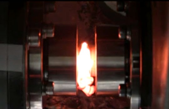
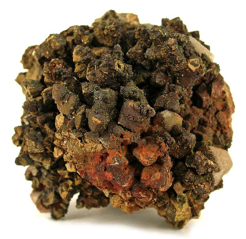

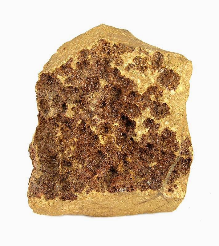

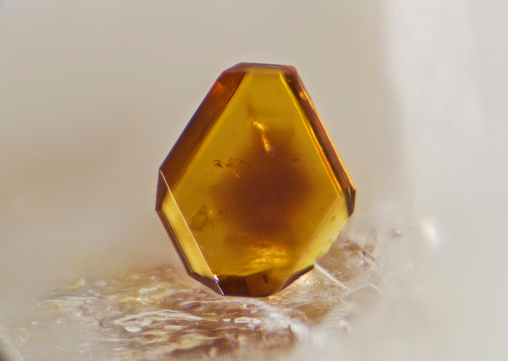
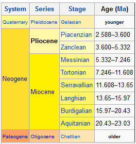
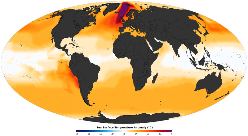
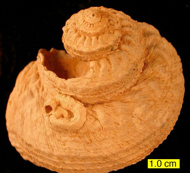
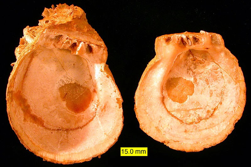
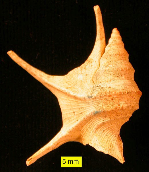
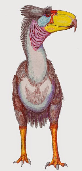
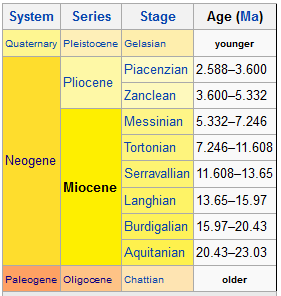
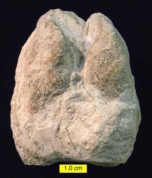
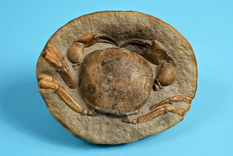
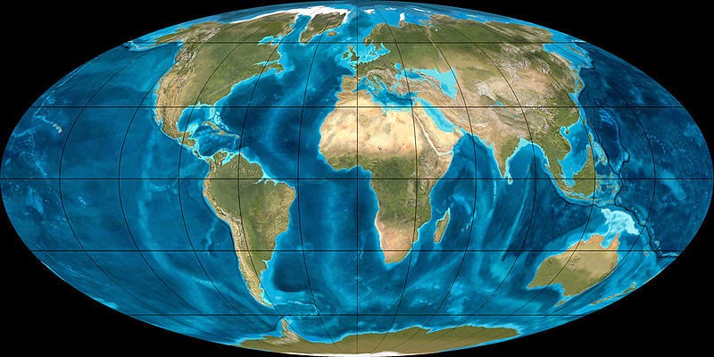
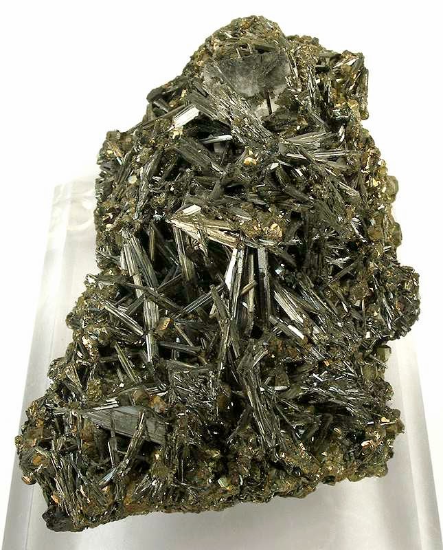
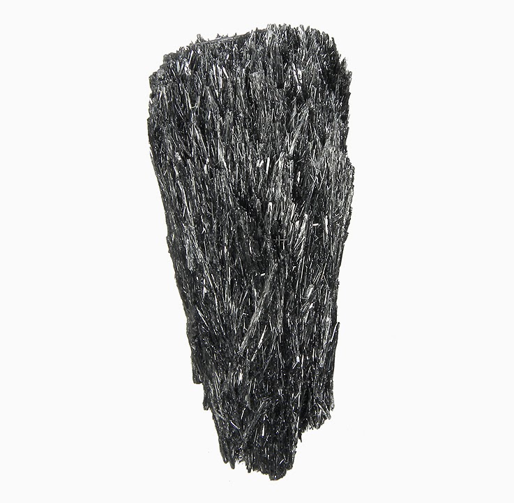
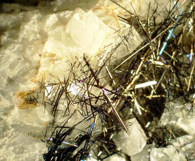
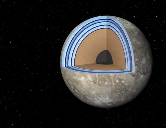
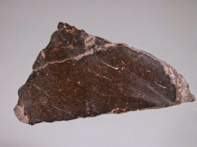
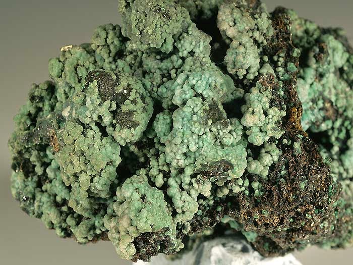
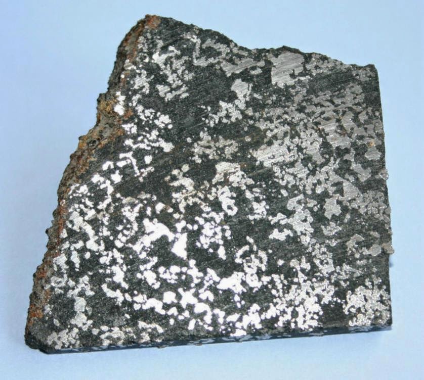
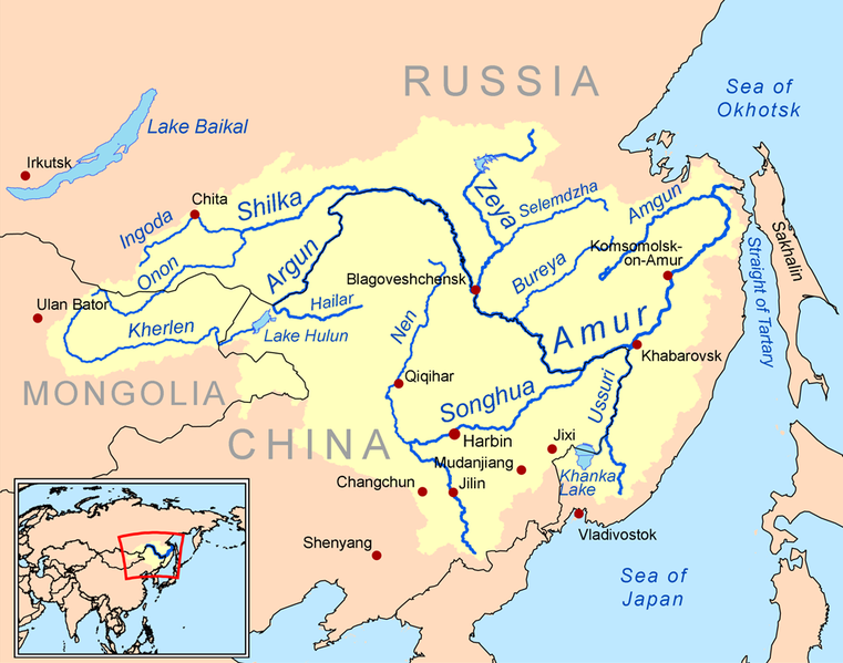
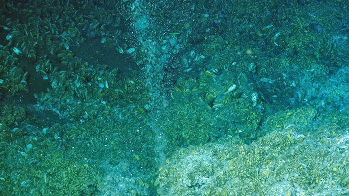
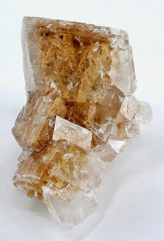
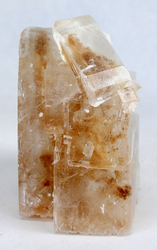
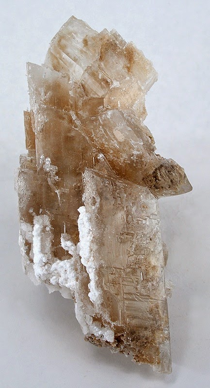
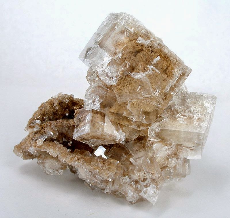
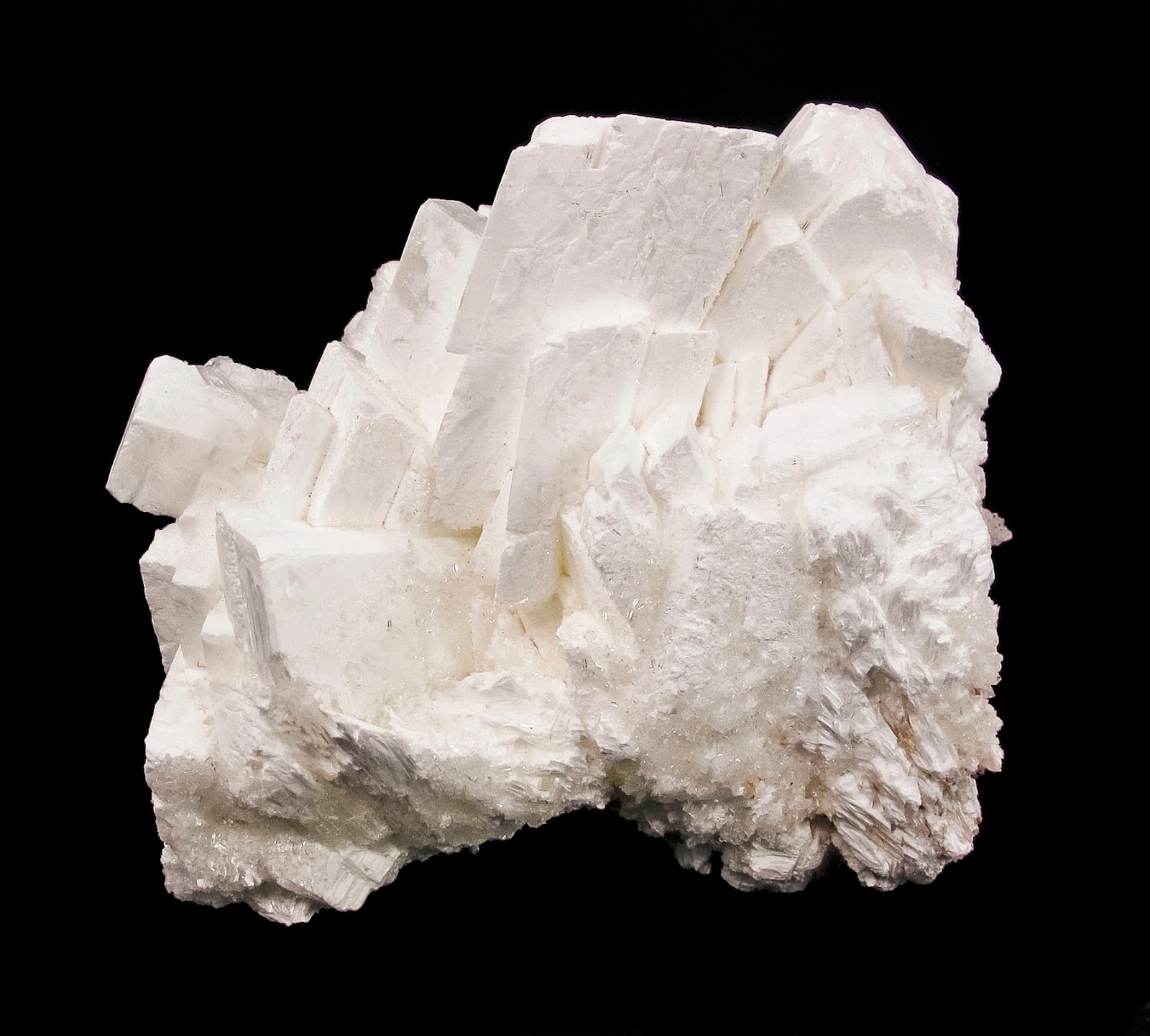
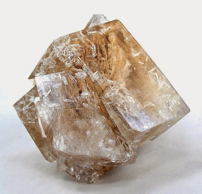
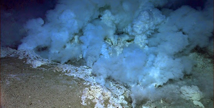

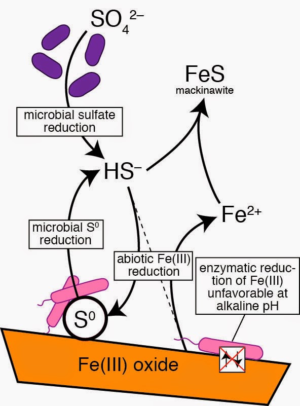
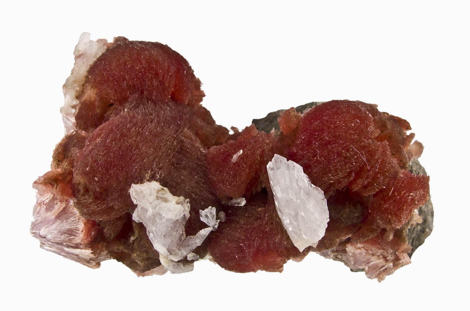
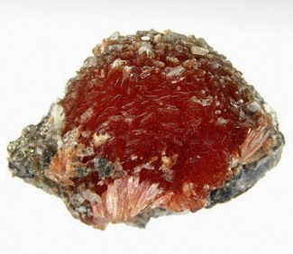
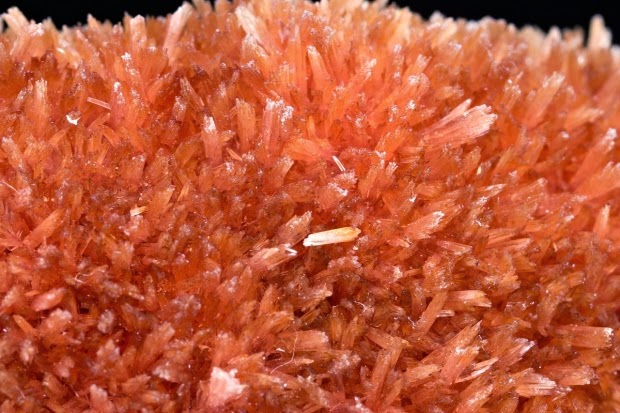
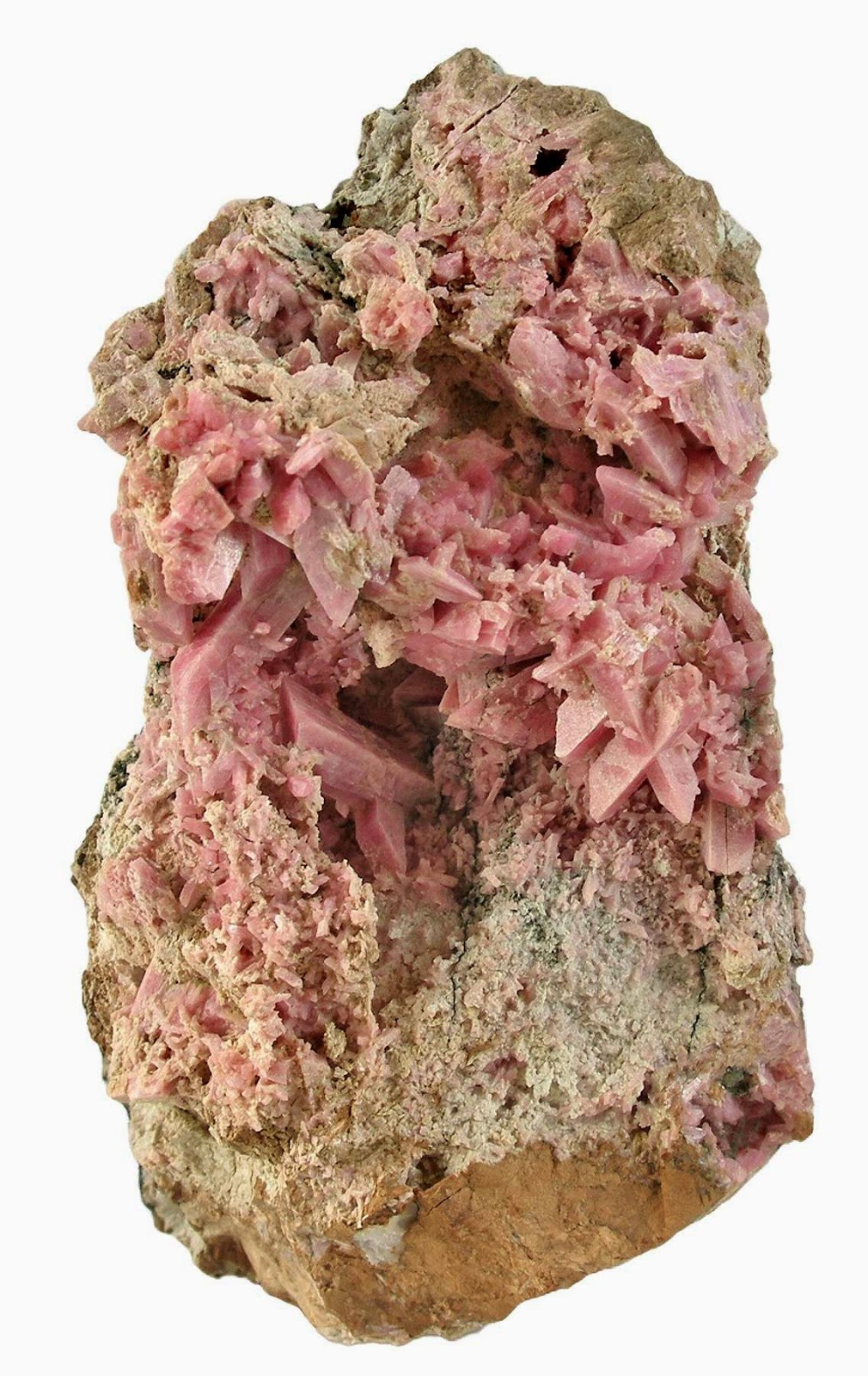
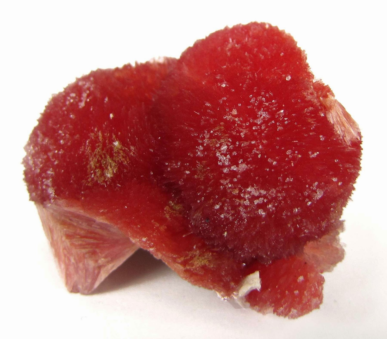
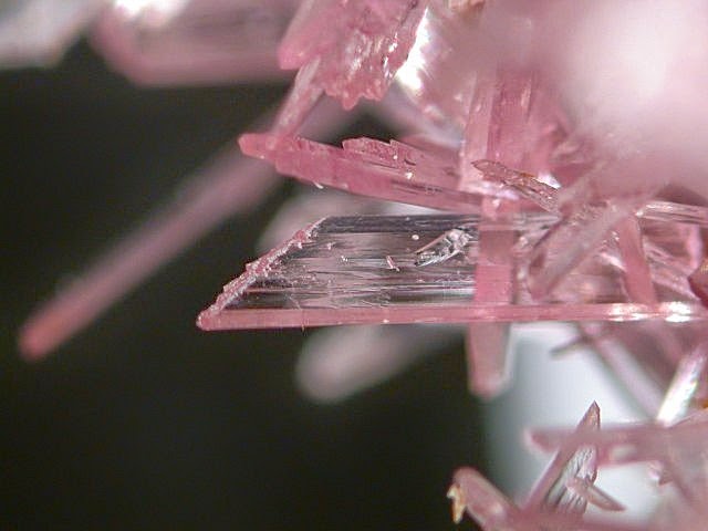

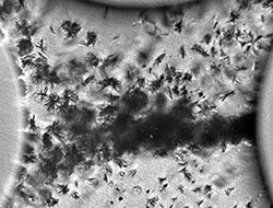
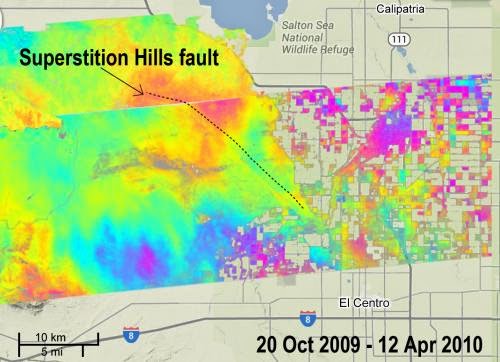
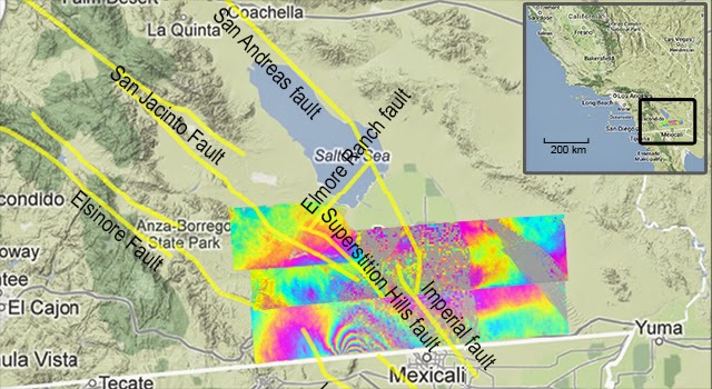
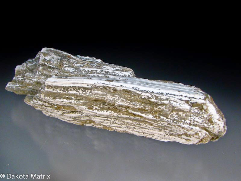
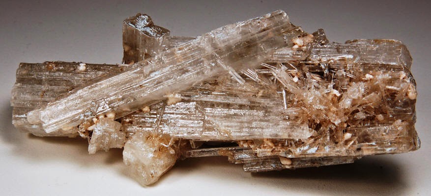
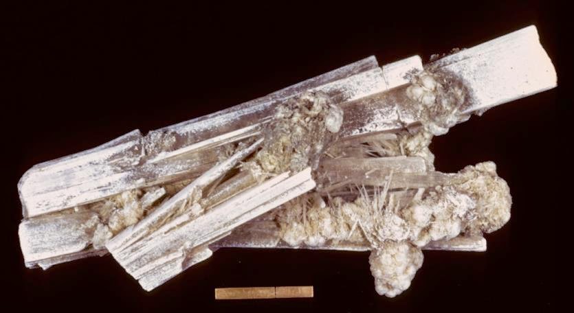
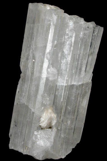
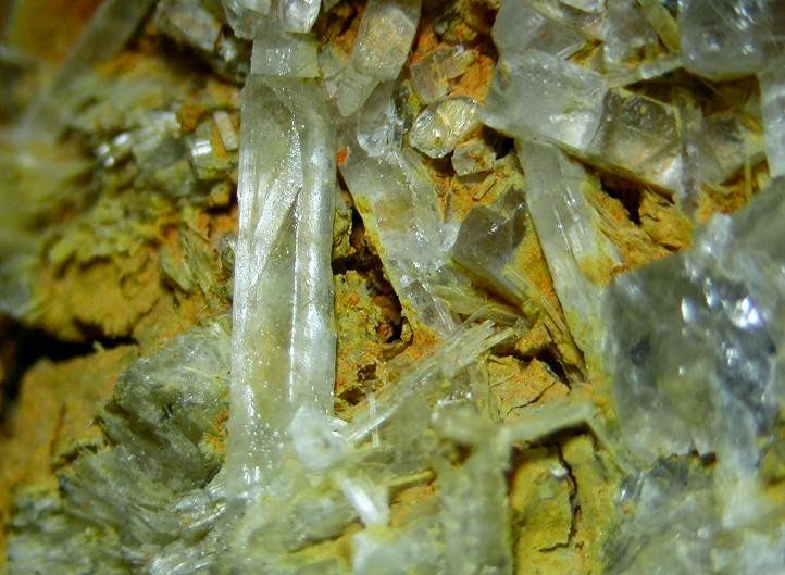
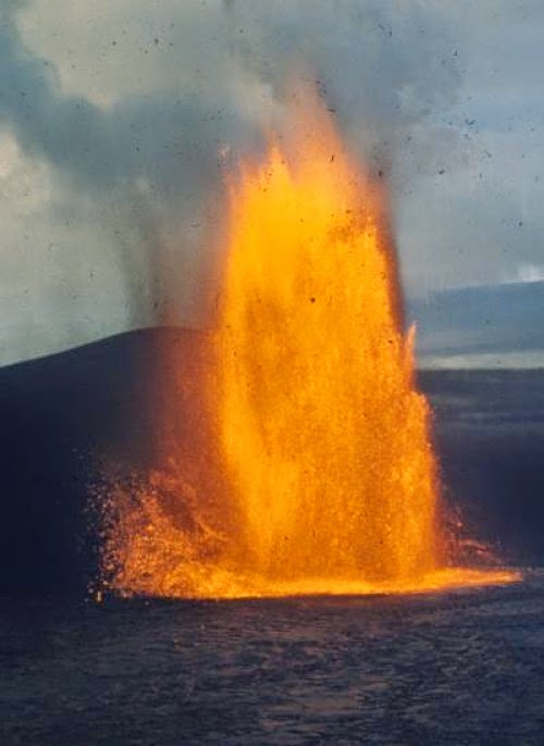
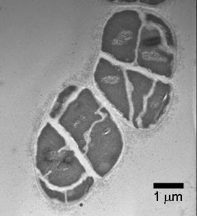
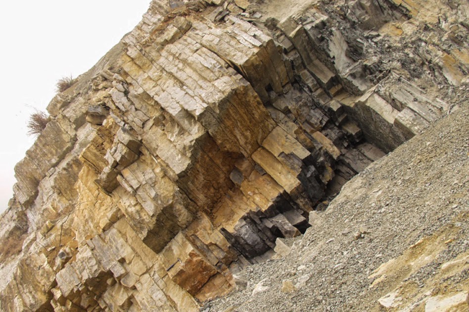