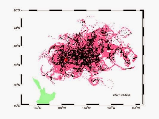
A team of scientists from the UK, the US, Australia and New Zealand have modelled the fate of a huge floating raft of volcanic rocks that formed in 2012 during a submarine eruption of a Pacific volcano.
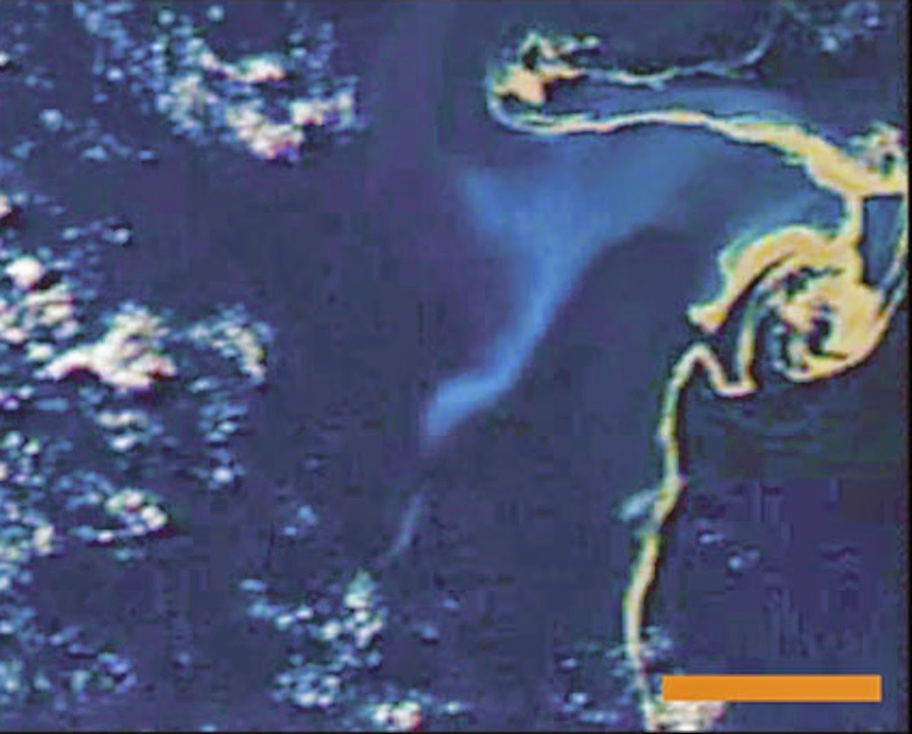
Described in this month’s edition of Nature Communications, they show how satellite images of the floating-rock raft’s passage across the Pacific can be used to test models of ocean circulation. Their results could be used to forecast the dispersal of future pumice (volcanic rock) islands, and protect shipping from the hazards they pose.
The eruptions of the Icelandic volcano, Eyjafjallajökull, in 2010 brought the hazards associated with volcanic ash sharply into focus. Air routes across northern Europe were disrupted, leaving many passengers stranded and far from home for days on end.
Ocean hazard
But hazards of floating islands of pumice spewed into the ocean from erupting volcanoes are less well-known.
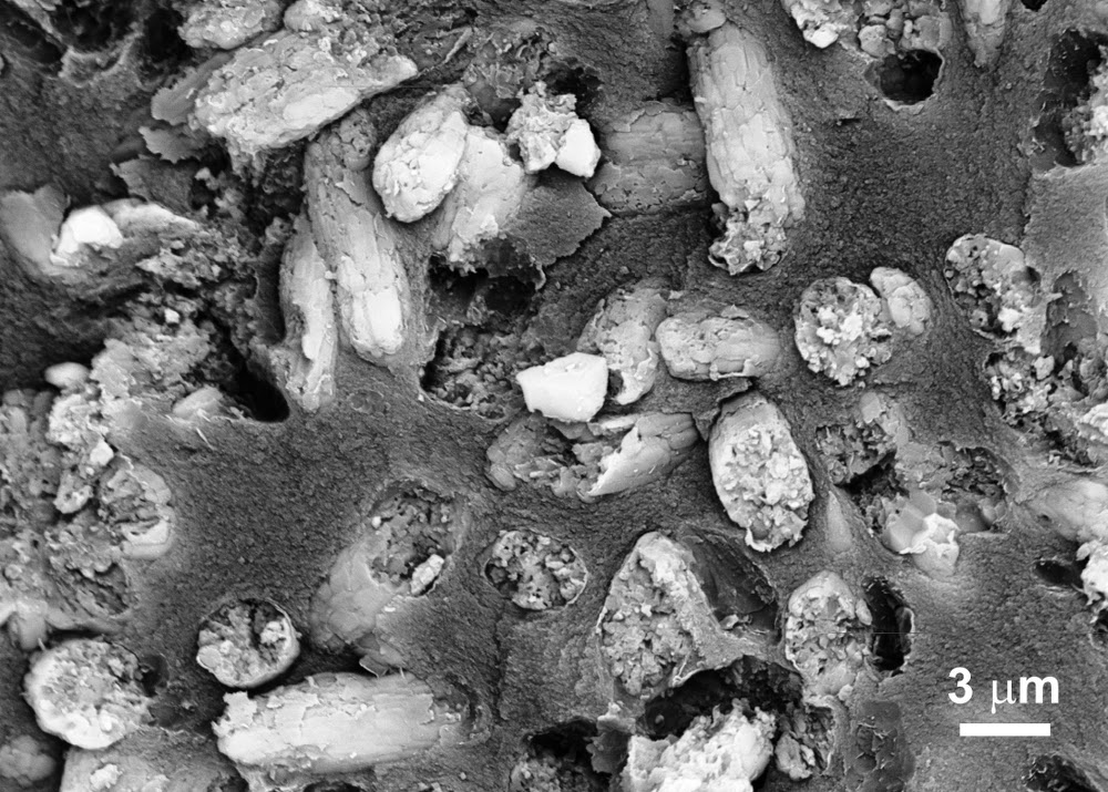
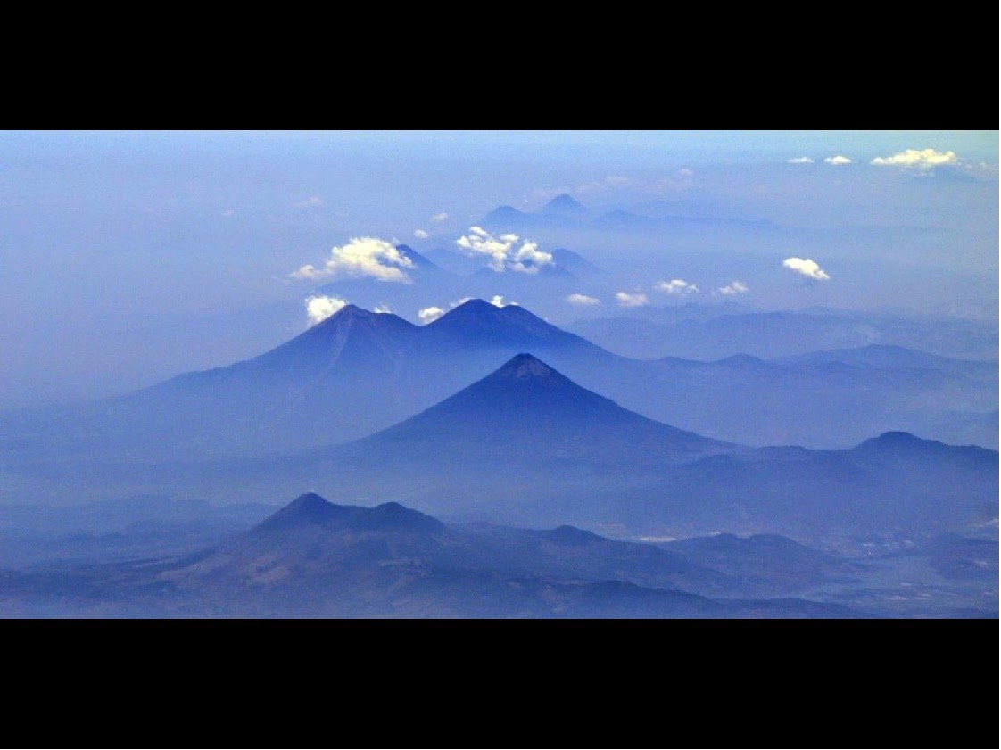
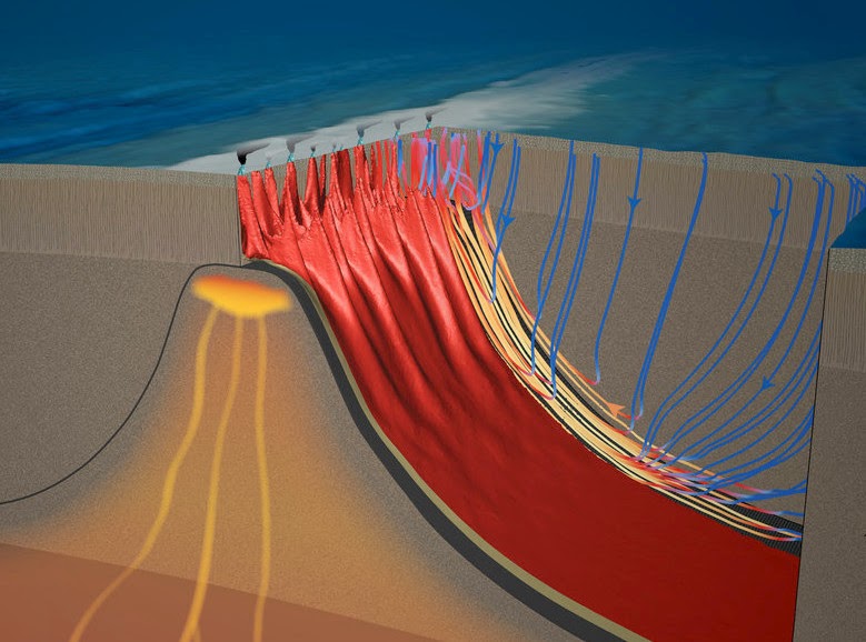
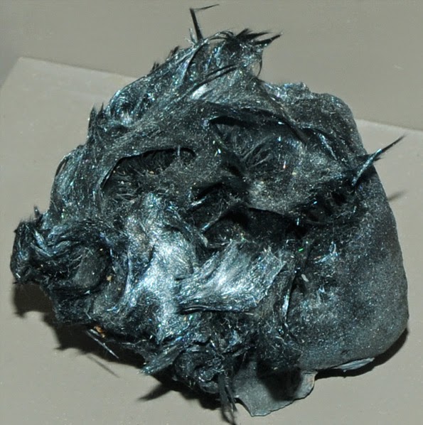
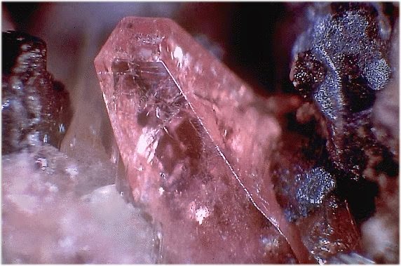
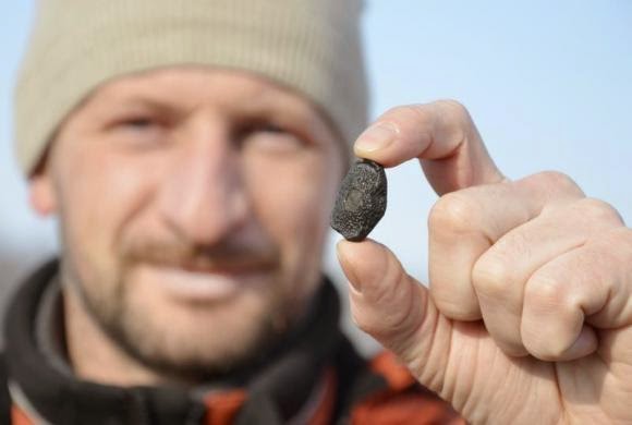
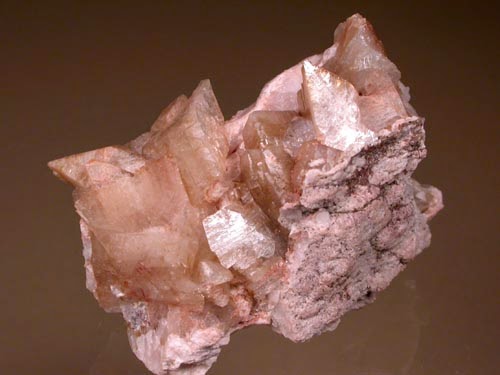
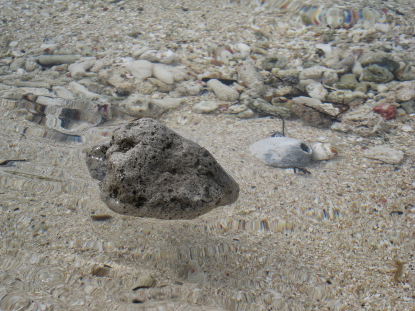
One such island grew from an explosion of the Havre volcano in the South Pacific, between Tonga and New Zealand, in July 2012. The volcano threw out a cubic kilometre of molten magma, which suddenly froze to form bubble-filled pumice.
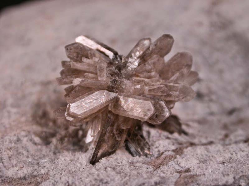
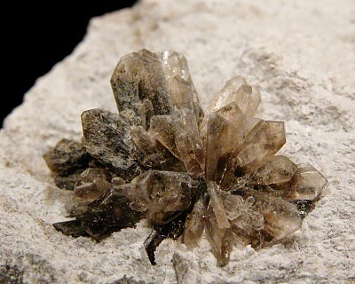
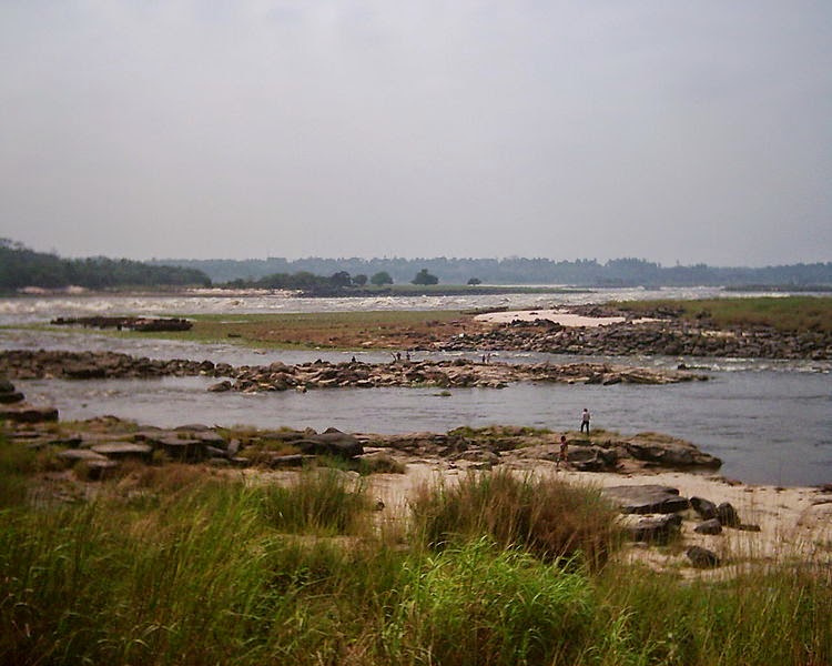
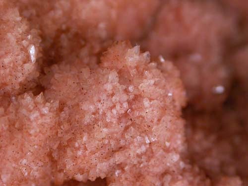
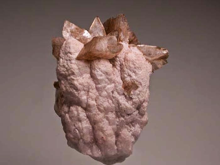
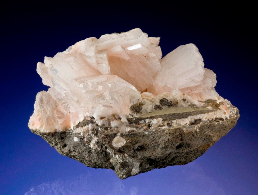
It is the bubbles trapped in pumice that make it so light – half the density of water – so the rock floats on water. Like natural flotsam, pebble to boulder-sized lumps of pumice clump together. This can create huge floating rafts in the seas around erupting volcanoes, and they can be tens of centimetres thick but thousands of kilometres in length.
Records of the use of pumice exist since the time of the Romans and Ancient Greeks. Its rough texture made them effective abrasives to remove dead skin from calluses and corns.
However, today, such floating pumice can pose a hazard for shipping. Hulls can be damaged by abrasion from the hard but light pumice, and when it approaches land these pumice rafts can block harbours and disrupt navigation.
Havre’s pumice island affected an area of ocean twice as big as both islands of New Zealand put together, floating atop the sea. Boats entering the volcanic debris reported engine problems, as the rock and dust clogged their water cooling intakes.
Threat to ocean life
It is not just the effects on shipping that have been a worry. The rafts of pumice stones block the sunlight from reaching plankton in the seas beneath. These plankton form the base of food chain when they convert sunlight to food through photosynthesis, and can be severely affected by floating pumice.
Floating rocks can also act as ferries for exotic invading species, such as shellfish and other organisms that make them their floating home. Indeed, it has been speculated that pumice islands like these were the first home that early life on Earth could have clung to and sprung from.
The study, led by Martin Jutzeler at the National Oceanography Centre in Southampton, UK, shows how the rafts eventually break up into ribbons of rock that can cover a wide area. The simulation techniques that the team has developed will allow the progress of future volcanic rafts to be predicted, and warnings issued to shipping, in the same way as volcanic ash clouds can be forecast for aircraft approaching stratospheric eruptions.
Note : The above story is based on materials provided by The Conversation
This story is published courtesy of The Conversation (under Creative Commons-Attribution/No derivatives). The above story is based on materials provided by