Parts of ancient Antarctica were as warm as today’s California coast, and polar regions of the southern Pacific Ocean registered 21st-century Florida heat, according to scientists using a new way to measure past temperatures.
But it wasn’t always that way, and the new measurements can help improve climate models used for predicting future climate, according to co-author Hagit Affek of Yale, associate professor of geology & geophysics.
“Quantifying past temperatures helps us understand ancient Antarctica were as warm as today’s California coast, and polar regions of the southern Pacific Ocean registered 21st-century Florida heat, according to scientists using a new way to measure past temperatures.
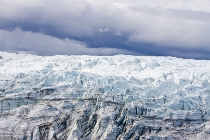
The findings, published the week of April 21 in the Proceedings of the National Academy of Sciences, underscore the potential for increased warmth at Earth’s poles and the associated risk of melting polar ice and rising sea levels, the researchers said.
Led by scientists at Yale, the study focused on Antarctica during the Eocene epoch, 40-50 million years ago, a period with high concentrations of atmospheric CO2 and consequently a greenhouse climate.
the sensitivity of the climate system to greenhouse gases, and especially the amplification of global warming in polar regions,” Affek said.
The paper’s lead author, Peter M.J. Douglas, performed the research as a graduate student in Affek’s Yale laboratory. He is now a postdoctoral scholar at the California Institute of Technology. The research team included paleontologists, geochemists, and a climate physicist.
By measuring concentrations of rare isotopes in ancient fossil shells, the scientists found that temperatures in parts of Antarctica reached as high as 17 degrees Celsius (63F) during the Eocene, with an average of 14 degrees Celsius (57F) — similar to the average annual temperature off the coast of California today.
Eocene temperatures in parts of the southern Pacific Ocean measured 22 degrees Centigrade (or about 72F), researchers said — similar to seawater temperatures near Florida today.
Today the average annual South Pacific sea temperature near Antarctica is about 0 degrees Celsius.
These ancient ocean temperatures were not uniformly distributed throughout the Antarctic ocean regions — they were higher on the South Pacific side of Antarctica — and researchers say this finding suggests that ocean currents led to a temperature difference.
“By measuring past temperatures in different parts of Antarctica, this study gives us a clearer perspective of just how warm Antarctica was when the Earth’s atmosphere contained much more CO2 than it does today,” said Douglas. “We now know that it was warm across the continent, but also that some parts were considerably warmer than others. This provides strong evidence that global warming is especially pronounced close to the Earth’s poles. Warming in these regions has significant consequences for climate well beyond the high latitudes due to ocean circulation and melting of polar ice that leads to sea level rise.”
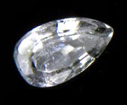
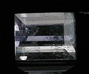
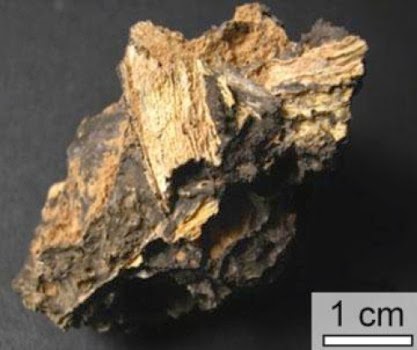
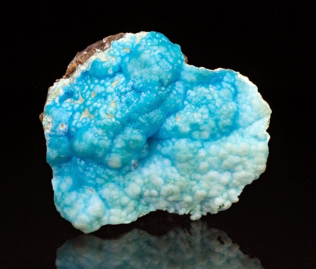
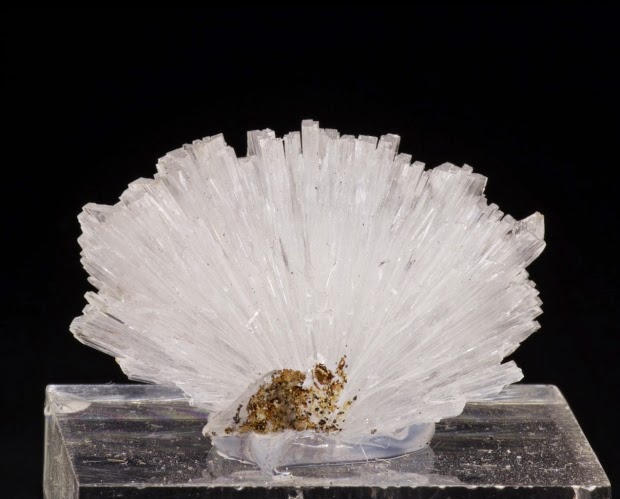
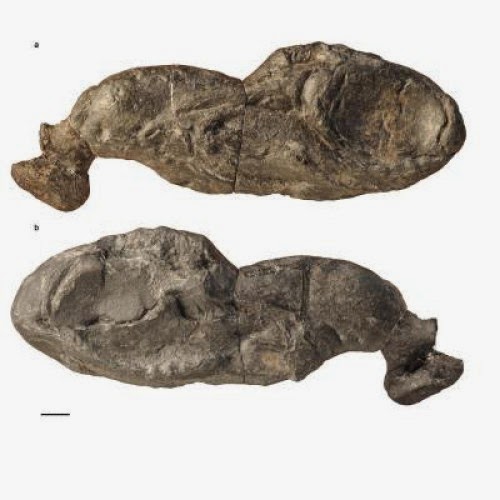
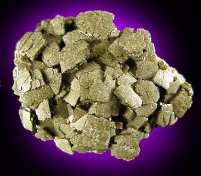
To determine the ancient temperatures, the scientists measured the abundance of two rare isotopes bound to each other in fossil bivalve shells collected by co-author Linda Ivany of Syracuse University at Seymour Island, a small island off the northeast side of the Antarctic Peninsula. The concentration of bonds between carbon-13 and oxygen-18 reflect the temperature in which the shells grew, the researchers said. They combined these results with other geo-thermometers and model simulations.
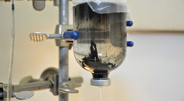
The new measurement technique is called carbonate clumped isotope thermometry.
“We managed to combine data from a variety of geochemical techniques on past environmental conditions with climate model simulations to learn something new about how the Earth’s climate system works under conditions different from its current state,” Affek said. “This combined result provides a fuller picture than either approach could on its own.”
Support for the research was provided by the National Science Foundation, Statoil, and the European Research Council.
Note : The above story is based on materials provided by Yale University.