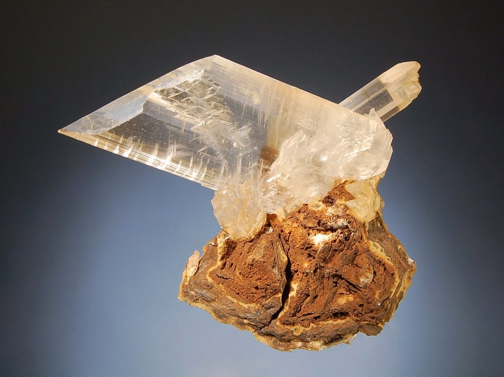
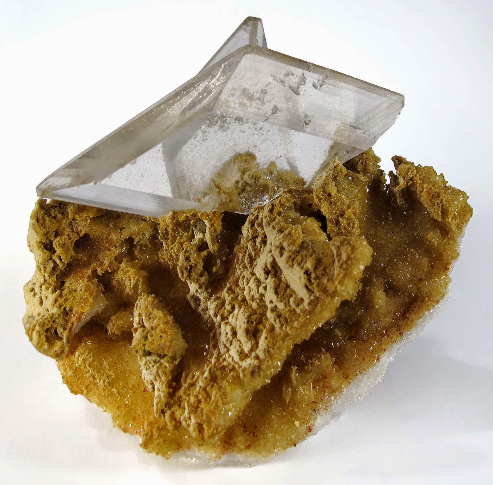
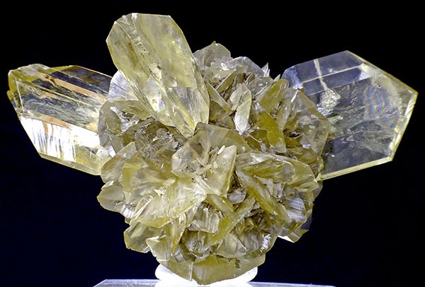
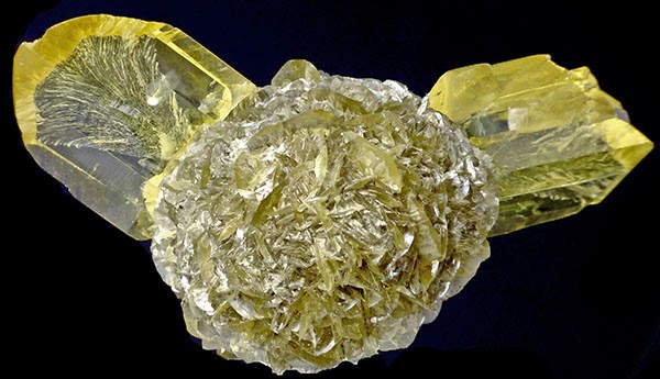
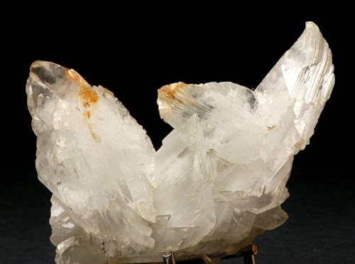
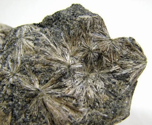
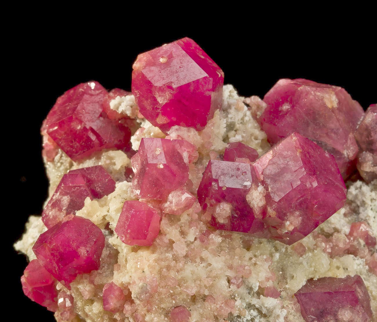
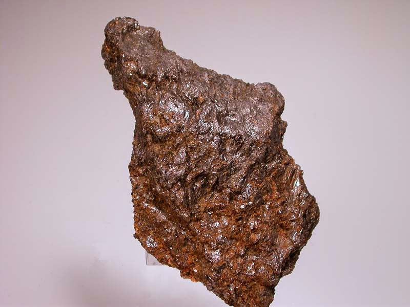
Chemical Formula: CaSO4·2H2O Locality: Numerous localities worldwide. Naica, Chihuahua, Mexico. Name Origin: From the Greek, gyps meaning “burned” mineral. Selenite from the Greek in allusion to its pearly luster (moon light) on cleavage fragments.
Gypsum is a soft sulfate mineral composed of calcium sulfate dihydrate, with the chemical formula CaSO4·2H2O. It can be used as a fertilizer, is the main constituent in many forms of plaster and is widely mined. A massive fine-grained white or lightly tinted variety of gypsum, called alabaster, has been used for sculpture by many cultures including Ancient Egypt, Mesopotamia, Ancient Rome, Byzantine empire and the Nottingham alabasters of medieval England. It is the definition of a hardness of 2 on the Mohs scale of mineral hardness. It forms as an evaporite mineral and as a hydration product of anhydrite.
Physical Properties
Cleavage: {010} Perfect, {100} Distinct, {011} Distinct Color: White, Colorless, Yellowish white, Greenish white, Brown. Density: 2.3 Diaphaneity: Transparent to translucent Fracture: Fibrous – Thin, elongated fractures produced by crystal forms or intersecting cleavages (e.g. asbestos). Hardness: 2 – Gypsum Luminescence: Fluorescent and phosphorescent, Short UV=orange yellow, Long UV=orange yellow. Luster: Pearly Streak: white
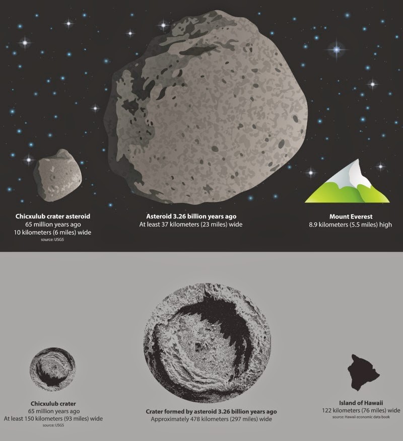
A graphical representation of the size of the asteroid thought to have killed the dinosaurs, and the crater it created, compared to an asteroid thought to have hit the Earth 3.26 billion years ago and the size of the crater it may have generated. A new study reveals the power and scale of the event some 3.26 billion years ago which scientists think created geological features found in a South African region known as the Barberton greenstone belt. Credit: Image courtesy of American Geophysical Union
Picture this: A massive asteroid almost as wide as Rhode Island and about three to five times larger than the rock thought to have wiped out the dinosaurs slams into Earth. The collision punches a crater into the planet’s crust that’s nearly 500 kilometers (about 300 miles) across: greater than the distance from Washington, D.C. to New York City, and up to two and a half times larger in diameter than the hole formed by the dinosaur-killing asteroid. Seismic waves bigger than any recorded earthquakes shake the planet for about half an hour at any one location — about six times longer than the huge earthquake that struck Japan three years ago. The impact also sets off tsunamis many times deeper than the one that followed the Japanese quake.
Although scientists had previously hypothesized enormous ancient impacts, much greater than the one that may have eliminated the dinosaurs 65 million years ago, now a new study reveals the power and scale of a cataclysmic event some 3.26 billion years ago which is thought to have created geological features found in a South African region known as the Barberton greenstone belt. The research has been accepted for publication in Geochemistry, Geophysics, Geosystems, a journal of the American Geophysical Union.
The huge impactor — between 37 and 58 kilometers (23 to 36 miles) wide — collided with the planet at 20 kilometers per second (12 miles per second). The jolt, bigger than a 10.8 magnitude earthquake, propelled seismic waves hundreds of kilometers through Earth, breaking rocks and setting off other large earthquakes. Tsunamis thousands of meters deep — far bigger than recent tsunamis generated by earthquakes — swept across the oceans that covered most of Earth at that time.
“We knew it was big, but we didn’t know how big,” Donald Lowe, a geologist at Stanford University and a co-author of the study, said of the asteroid.
Lowe, who discovered telltale rock formations in the Barberton greenstone a decade ago, thought their structure smacked of an asteroid impact. The new research models for the first time how big the asteroid was and the effect it had on the planet, including the possible initiation of a more modern plate tectonic system that is seen in the region, according to Lowe.
The study marks the first time scientists have mapped in this way an impact that occurred more than 3 billion years ago, Lowe added, and is likely one of the first times anyone has modeled any impact that occurred during this period of Earth’s evolution.
The impact would have been catastrophic to the surface environment. The smaller, dino-killing asteroid crash is estimated to have released more than a billion times more energy than the bombs that destroyed Hiroshima and Nagasaki. The more ancient hit now coming to light would have released much more energy, experts said.
The sky would have become red hot, the atmosphere would have been filled with dust and the tops of oceans would have boiled, the researchers said. The impact sent vaporized rock into the atmosphere, which encircled the globe and condensed into liquid droplets before solidifying and falling to the surface, according to the researchers.
The impact may have been one of dozens of huge asteroids that scientists think hit Earth during the tail end of the Late Heavy Bombardment period, a major period of impacts that occurred early in Earth’s history — around 3 billion to 4 billion years ago.
Many of the sites where these asteroids landed were destroyed by erosion, movement Earth’s crust and other forces as Earth evolved, but geologists have found a handful of areas in South Africa, and Western Australia that still harbor evidence of these impacts that occurred between 3.23 billion and 3.47 billion years ago. The study’s co-authors think the asteroid hit Earth thousands of kilometers away from the Barberton Greenstone Belt, although they can’t pinpoint the exact location.
“We can’t go to the impact sites. In order to better understand how big it was and its effect we need studies like this,” said Lowe. Scientists must use the geological evidence of these impacts to piece together what happened to the Earth during this time, he said.
The study’s findings have important implications for understanding the early Earth and how the planet formed. The impact may have disrupted Earth’s crust and the tectonic regime that characterized the early planet, leading to the start of a more modern plate tectonic system, according to the paper’s co-authors.
The pummeling the planet endured was “much larger than any ordinary earthquake,” said Norman Sleep, a physicist at Stanford University and co-author of the study. He used physics, models, and knowledge about the formations in the Barberton greenstone belt, other earthquakes and other asteroid impact sites on Earth and the moon to calculate the strength and duration of the shaking that the asteroid produced. Using this information, Sleep recreated how waves traveled from the impact site to the Barberton greenstone belt and caused the geological formations.
The geological evidence found in the Barberton that the paper investigates indicates that the asteroid was “far larger than anything in the last billion years,” said Jay Melosh, a professor at Purdue University in West Lafayette, Indiana, who was not involved in the research.
The Barberton greenstone belt is an area 100 kilometers (62 miles) long and 60 kilometers (37 miles) wide that sits east of Johannesburg near the border with Swaziland. It contains some of the oldest rocks on the planet.
The model provides evidence for the rock formations and crustal fractures that scientists have discovered in the Barberton greenstone belt, said Frank Kyte, a geologist at UCLA who was not involved in the study.
“This is providing significant support for the idea that the impact may have been responsible for this major shift in tectonics,” he said.
Reconstructing the asteroid’s impact could also help scientists better understand the conditions under which early life on the planet evolved, the paper’s authors said. Along with altering Earth itself, the environmental changes triggered by the impact may have wiped out many microscopic organisms living on the developing planet, allowing other organisms to evolve, they said.
“We are trying to understand the forces that shaped our planet early in its evolution and the environments in which life evolved,” Lowe said.
Note : The above story is based on materials provided by American Geophysical Union.
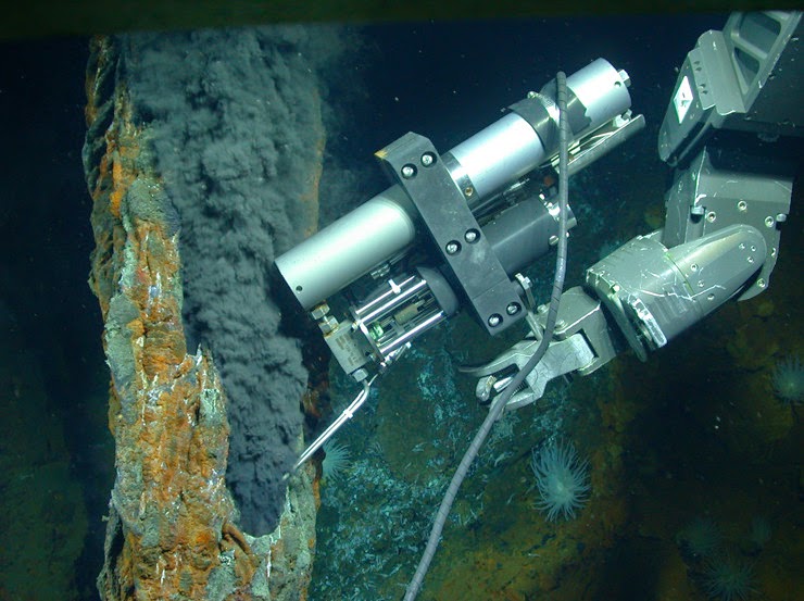
Making methanethiol from the chemicals available in hydrothermal black smoker fluids was thought to have been an easy process. To test this theory, the researchers collected fluids in isobaric gas-tight samplers (IGTs) from black smokers and analyzed them for the presence of methanethiol. Credit: Chris German, Woods Hole Oceanographic Institution
One of the greatest mysteries facing humans is how life originated on Earth. Scientists have determined approximately when life began (roughly 3.8 billion years ago), but there is still intense debate about exactly how life began. One possibility — that simple metabolic reactions emerged near ancient seafloor hot springs, enabling the leap from a non-living to a living world — has grown in popularity in the last two decades.
Recent research by geochemists Eoghan Reeves, Jeff Seewald, and Jill McDermott at Woods Hole Oceanographic Institution (WHOI) is the first to test a fundamental assumption of this ‘metabolism first’ hypothesis, and finds that it may not have been as easy as previously assumed. Instead, their findings could provide a focus for the search for life on other planets. The work is published in Proceedings of the National Academy of Sciences.
In 1977, scientists discovered biological communities unexpectedly living around seafloor hydrothermal vents, far from sunlight and thriving on a chemical soup rich in hydrogen, carbon dioxide, and sulfur, spewing from the geysers. Inspired by these findings, scientists later proposed that hydrothermal vents provided an ideal environment with all the ingredients needed for microbial life to emerge on early Earth. A central figure in this hypothesis is a simple sulfur-containing carbon compound called “methanethiol” — a supposed geologic precursor of the Acetyl-CoA enzyme present in many organisms, including humans. Scientists suspected methanethiol could have been the “starter dough” from which all life emerged.
The question Reeves and his colleagues set out to test was whether methanethiol — a critical precursor of life — could form at modern day vent sites by purely chemical means without the involvement of life. Could methanethiol be the bridge between a chemical, non-living world and the first microbial life on the planet?
Carbon dioxide, hydrogen and sulfide are the common ingredients present in hydrothermal black smoker fluids. “The thought was that making methanethiol from these basic ingredients at seafloor hydrothermal vents should therefore have been an easy process,” adds Reeves.
The theory was appealing, and solved many of the basic problems with existing ideas that life may have been carried to Earth on a comet or asteroid; or that genetic material emerged first — the “RNA World” hypothesis. However, says Reeves, “it’s taken us a while to get out there and actually start to test this ‘metabolism first’ idea in the natural environment, by using modern vents as analogs for those that were around when life first began.”
And when they did get out there, the scientists were surprised by what they found.
To directly measure methanethiol, the researchers went to hydrothermal vent sites where the chemistry predicted they would find abundant methanethiol, and others where very little was predicted to form. In total, they measured the distribution of methanethiol in 38 hydrothermal fluids from multiple differing geologic environments including systems along the Mid-Atlantic Ridge, Guaymas Basin, the East Pacific Rise, and the Mid-Cayman Rise over a period between 2008 and 2012.
“Some systems are very rich in hydrogen, and when you have a lot of hydrogen it should, in theory, be very easy to make a lot of methanethiol,” says Reeves. The fluids were collected in isobaric gas-tight samplers (IGTs) developed by Jeffrey Seewald, which maintain fluids at their natural pressure and allow for dissolved gas analyses.
Instead of an abundance of methanethiol, the data they collected in the hydrogen-rich environments showed very little was present. “We actually found that it doesn’t matter how much hydrogen you have in black smoker fluids, you don’t seem to be making a lot of methanethiol where you should be making a lot of it,” Reeves says. Surprisingly, in the low-hydrogen environments, where much less should form, the research actually found more methanethiol than they had predicted, contradicting the original idea of how methanethiol forms. Overall, this means that jump-starting proto-metabolic reactions in hydrogen-rich early Earth hydrothermal systems through carbon-sulfur chemistry would likely have been much harder than many had assumed.
Critically, the researchers found an abundance of methanethiol being formed in low temperature fluids (below about 200°C), where hot black smoker fluid mixes with colder sea water beneath the seafloor. The presence of other telltale markers in these fluids, such as ammonia — a byproduct of biomass breakdown — strongly suggests these fluids are ‘cooking’ existing microbial organic matter. The breakdown of existing subseafloor life when conditions get too hot may therefore be responsible for producing large amounts of methanethiol.
“What we essentially found in our survey is that we don’t think methanethiol is forming by purely chemical means without the involvement of life. This might be disappointing news for anyone assuming an easy start for hydrothermal proto-metabolism,” says Reeves. “However, our finding that methanethiol may be readily forming as a breakdown product of microbial life provides further indication that life is present and widespread below the seafloor and is very exciting.”
The researchers believe this new understanding could change how we think about searching for life on other planets. “The upside is, now we have a pretty simple marker for life. Someday if we can land a rover on the ice-covered oceans of Jupiter’s moon Europa — another place in the Solar System that may host hydrothermal vents, and possibly life — and successfully drill through the ice, the first thing it should probably try to measure is methanethiol,” Reeves says. “This is already something scientists are thinking about, and it is exciting to think this might even happen in our life time.”
As for the search for the origins of life, Reeves agrees that hydrothermal vents are still a very favorable place for life to emerge, but, he says, “maybe methanethiol just wasn’t a good starter dough. The hydrothermal environment is still a perfect place to support early life, and the question of how it all started is still open.”
This research was supported by grants from the National Science Foundation and NASA. Additional funds were provided by the WHOI Deep Ocean Exploration Institute, InterRidge, and the Deutsche Forschungsgemeinschaft Research Center/Cluster of Excellence MARUM “The Ocean in the Earth System” (E.P.R.).
Note : The above story is based on materials provided by Woods Hole Oceanographic Institution.
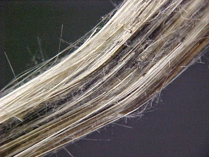
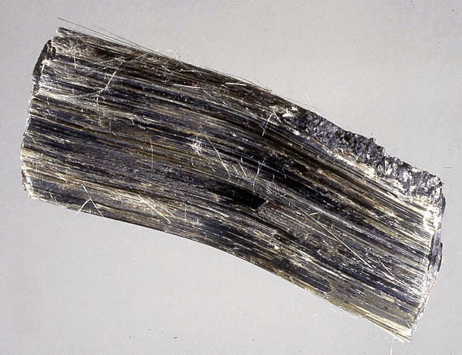
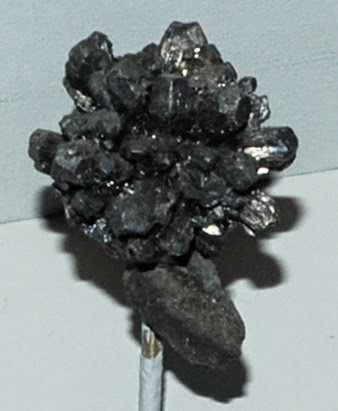
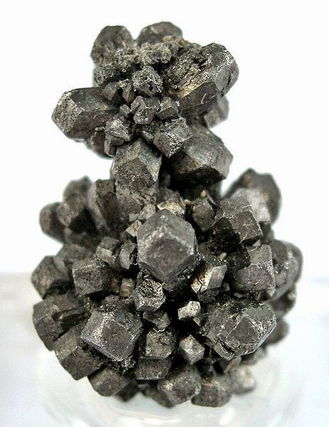
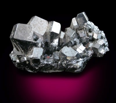
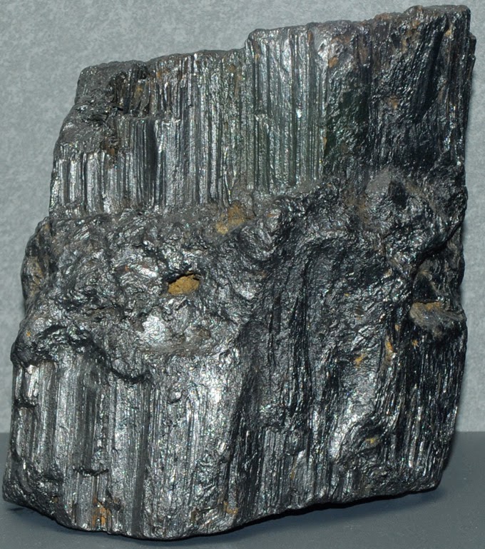
Chemical Formula: Fe7Si8O22(OH)2 Name Origin: Named for Louis Emmanuel Gruner (1809-1883), Swiss-French chemist who analyzed the mineral.
Grunerite is a mineral of the amphibole group of minerals with formula Fe7Si8O22(OH)2. It is the iron endmember of the grunerite-cummingtonite series. It forms as fibrous, columnar or massive aggregates of crystals. The crystals are monoclinic prismatic. The luster is glassy to pearly with colors ranging from green, brown to dark grey. The Mohs hardness is 5 to 6 and the specific gravity is 3.4 to 3.5.
It was discovered in 1853 and named after Emmanuel-Louis Gruner (1809–1883), a Swiss-French chemist who first analysed it.
Physical Properties
Cleavage: {110} Perfect, {???} Distinct Color: Ashen, Brown, Brownish green, Dark gray. Density: 3.4 – 3.5, Average = 3.45 Diaphaneity: Translucent to opaque Fracture: Sub Conchoidal – Fractures developed in brittle materials characterized by semi-curving surfaces. Hardness: 5-6 – Between Apatite and Orthoclase Luminescence: Non-fluorescent. Luster: Vitreous – Pearly Streak: colorless
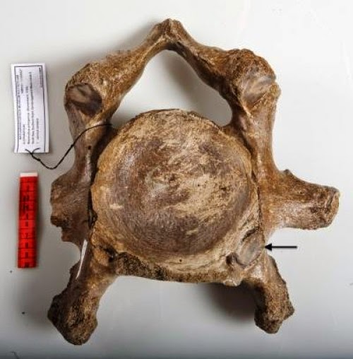
The arrow indicates a large articulation facet of a cervical rib on a fossil cervical vertebra of a woolly mammoth of the Natural History Museum Rotterdam. Credit: Joris van Alphen
Researchers recently noticed that the remains of woolly mammoths from the North Sea often possess a ‘cervical’ (neck) rib — in fact, 10 times more frequently than in modern elephants (33.3% versus 3.3%). In modern animals, these cervical ribs are often associated with inbreeding and adverse environmental conditions during pregnancy. If the same factors were behind the anomalies in mammoths, this reproductive stress could have further pushed declining mammoth populations towards ultimate extinction.
Mammals, even the long-necked giraffes and the short-necked dolphins, almost always have seven neck vertebrae (exceptions being sloths, manatees and dugongs), and these vertebrae do not normally possess a rib. Therefore, the presence of a ‘cervical rib’ (a rib attached to a cervical vertebra) is an unusual event, and is cause for further investigation. A cervical rib itself is relatively harmless, but its development often follows genetic or environmental disturbances during early embryonic development. As a result, cervical ribs in most mammals are strongly associated with stillbirths and multiple congenital abnormalities that negatively impact the lifespan of an individual.
Researchers from the Rotterdam Museum of Natural History and the Naturalis Biodiversity Center in Leiden examined mammoth and modern elephant neck vertebrae from several European museum collections. “It had aroused our curiosity to find two cervical vertebrae, with large articulation facets for ribs, in the mammoth samples recently dredged from the North Sea. We knew these were just about the last mammoths living there, so we suspected something was happening. Our work now shows that there was indeed a problem in this population,” said Jelle Reumer, one of the authors on the study published today in the open access journal PeerJ.
The incidence of abnormal cervical vertebrae in mammoths is much higher than in the modern sample, strongly suggesting a vulnerable condition in the species. Potential factors could include inbreeding (in what is assumed to have been an already small population) as well as harsh conditions such as disease, famine, or cold, all of which can lead to disturbances of embryonic and fetal development. Given the considerable birth defects that are associated with this condition, it is very possible that developmental abnormalities contributed towards the eventual extinction of these late Pleistocene mammoths.
The peer-reviewed study, entitled “Extraordinary incidence of cervical ribs indicates vulnerable condition in Late Pleistocene mammoths” was authored by Jelle Reumer of the Rotterdam Museum of Natural History and Clara ten Broek and Frietson Galis of Naturalis Biodiversity Center (Leiden).
Note : The above story is based on materials provided by PeerJ.
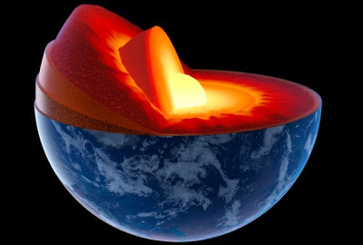
The contours of the Earth’s crust are influenced by the high temperatures deep within the Earth’s mantle, according to a new study published in Science. A team of researchers, led by Brown University, demonstrated that those temperature differences control the elevation and volcanic activity along mid-ocean ridges, the colossal mountain ranges that line the ocean floor.
Forming at the boundaries of tectonic plates, mid-ocean ridges circle the globe like seams on a baseball. Magma from deep within the Earth rises up to fill in the cracks between the plates as they move apart, creating fresh crust on the ocean floor as it cools. This new crust is thicker in some places than others, forming ridges with widely varying elevations. In some parts of the world, these ridges are deep in the ocean, miles beneath the surface. In other places such as Iceland, the ridge tops are exposed above the ocean’s surface.
“These variations in ridge depth require an explanation,” said Colleen Dalton, assistant professor of geological sciences at Brown. “Something is keeping them either sitting high or sitting low.”
The research team discovered that the “something” was the temperature of the rocks deep below the Earth’s surface.
At depths extending below 250 miles, the team was able to show that mantle temperatures along the ridges vary by as much as 250 degrees Celsius by analyzing the speeds of seismic waves generated by earthquakes. They found that, in general, higher points on the ridges are associated with higher temperatures, while lower points are associated with cooler temperatures. One unsurprising finding of this study is that volcanic hot spots along the ridges — such as volcanoes near Iceland, and the islands of Ascension and Tristan da Cunha — all sit above warm spots in the mantle.
“It is clear from our results that what’s being erupted at the ridges is controlled by temperature deep in the mantle,” Dalton told Brown University’s Kevin Stacey. “It resolves a long-standing controversy and has not been shown definitively before.”
The mid-ocean ridges function as a window to the interior of the planet for geologists by providing clues about the properties of the mantle below.
A thicker crust is suggested by a higher ridge elevation, indicating that a larger volume of magma erupted at the surface. The new study explains that this excess magma could have been caused by very hot temperatures in the mantle. The fact that hot mantle material is not the only way to produce excess magma, however, presents a challenge to this theory. The amount of melt is also controlled by the chemical composition of the mantle. Some rock compositions melt at lower temperatures, allowing for a larger volume of molten rock. Because of this, it has been unclear for the last several decades whether mid-ocean ridge elevations are caused by variations in the temperature of the mantle or variations in the rock composition of the mantle.
Dalton’s team introduced two additional data sets to help them distinguish between these two possible scenarios.
One data set was the chemistry of basalts, the rock that forms from the solidification of magma at the mid-ocean ridge. Basalt compositions can vary greatly depending on the temperature and composition of the mantle material from which they’re derived. To create this data set, the researchers analyzed almost 17,000 basalts formed along mid-ocean ridges worldwide.
Seismic wave tomography made up the second data set. During earthquakes, seismic waves pulse through the rock of the crust and the mantle. Scientists measure the velocity of those waves to gather data about the characteristics of the rocks through which they passed. “It’s like performing a CAT scan of the inside of the Earth,” Dalton added. Temperature has a great effect on seismic wave speeds, with waves propagating more quickly in cooler rocks than in hotter ones.
By comparing the seismic data from hundreds of earthquakes to data on elevation and rock chemistry from the ridges, the team found correlations which revealed that temperatures deep in the mantle varied between 1,300 and 1,550 degrees Celsius underneath about 38,000 miles of ridge terrain. “It turned out,” said Dalton, “that seismic tomography was the smoking gun. The only plausible explanation for the seismic wave speeds is a very large temperature range.”
The results demonstrated that as mantle temperatures fall, so too do ridge elevations. The hottest point beneath the ridges was found to be near Iceland — also the site of the ridges’ highest elevation — while the lowest temperatures were found near the lowest point, an area of very deep and rugged seafloor known as the Australian-Antarctic discordance in the Indian Ocean.
There has been a long-standing debate in the scientific community about whether a mantle plume — a vertical jet of hot rock originating from deep in the Earth — intersects the mid-ocean ridge in Iceland. The findings of this study provide strong support for this theory, as well as for mantle plumes being the culprit for the excess magma volume in all regions with above-average temperatures near volcanic hot spots.
The Earth’s mantle does not sit still, despite being made of solid rock. It is constantly undergoing convection, where material from the depths of the Earth churns towards the surface and back again.
“Convection is why we have plate tectonics and earthquakes,” Dalton said. “It’s also responsible for almost all volcanism at the surface. So understanding mantle convection is crucial to understanding many fundamental questions about the Earth.”
There are two main factors in the mechanism of convection: variations in the composition of the mantle and variations in its temperature. Dalton says that their findings point to temperature as a primary factor in how convection is expressed on the surface.
“We get consistent and coherent temperature measurements from the mantle from three independent datasets,” Dalton said. “All of them suggest that what we see at the surface is due to temperature, and that composition is only a secondary factor. What is surprising is that the data require the temperature variations to exist not only near the surface but also many hundreds of kilometers deep inside the Earth.”
Dalton says that the findings will be useful for future research using seismic waves because the temperature readings as indicated by seismology were backed up by the other datasets. This allows them to be used to calibrate seismic readings for places where geochemical samples aren’t available, allowing scientists to estimate temperature deep in the Earth’s mantle all over the globe.
Note : The above story is based on materials provided by April Flowers for redOrbit
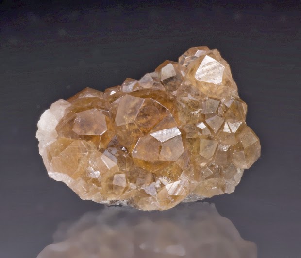
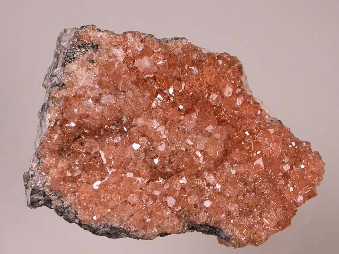
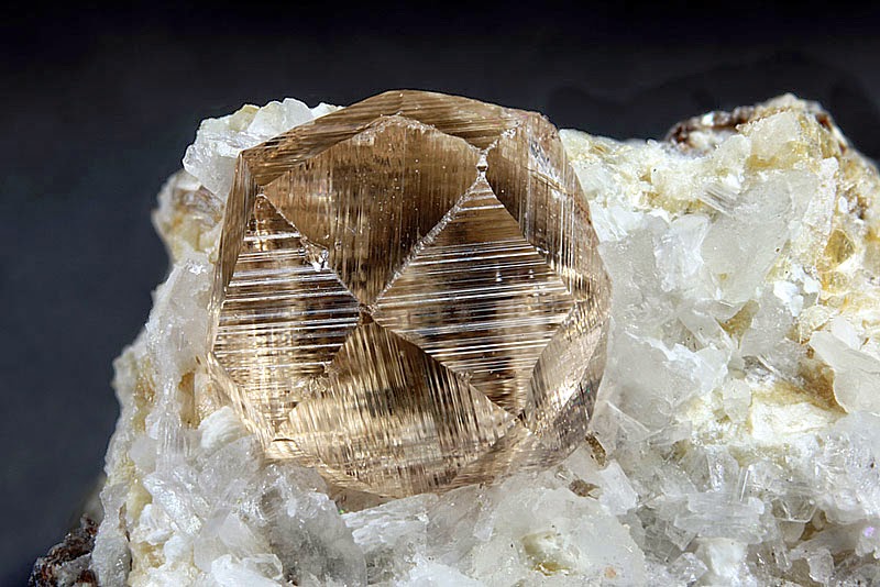
Chemical Formula: Ca3Al2(SiO4)3 Locality: Isle of Mull, Scotland. Name Origin: Grossular is from the Latin grossularia meaning “gooseberry.” Hessonite is from the Greek hesson, meaning “slight” in reference to the smaller specific gravity.
Grossular or grossularite is a calcium-aluminium mineral species of the garnet gemstone group with the formula Ca3Al2(SiO4)3, though the calcium may in part be replaced by ferrous iron and the aluminium by ferric iron. The name grossular is derived from the botanical name for the gooseberry, grossularia, in reference to the green garnet of this composition that is found in Siberia. Other shades include cinnamon brown (cinnamon stone variety), red, and yellow.
Physical Properties
Color: Brown, Colorless, Green, Gray, Yellow. Density: 3.42 – 3.72, Average = 3.57 Diaphaneity: Transparent to subtranslucent Fracture: Sub Conchoidal – Fractures developed in brittle materials characterized by semi-curving surfaces. Hardness: 6.5-7.5 Luminescence: Fluorescent, Short UV=pink, Long UV=orange. Luster: Vitreous – Resinous Streak: brownish white
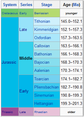
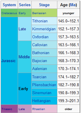
The Late Jurassic is the third epoch of the Jurassic Period, and it spans the geologic time from 161.2 ± 4.0 to 145.5 ± 4.0 million years ago (Ma), which is preserved in Upper Jurassic strata. In European lithostratigraphy, the name “Malm” indicates rocks of Late Jurassic age. In the past, this name was also used to indicate the unit of geological time, but this usage is now discouraged to make a clear distinction between lithostratigraphic and geochronologic/chronostratigraphic units.
Subdivisions
The Late Jurassic is divided into three ages, which correspond with the three (faunal) stages of Upper Jurassic rock:
Tithonian (150.8 ± 4.0 – 145.5 ± 4.0 Ma)
Kimmeridgian (155.7 ± 4.0 – 150.8 ± 4.0 Ma)
Oxfordian (161.2 ± 4.0 – 155.7 ± 4.0 Ma)
Paleogeography
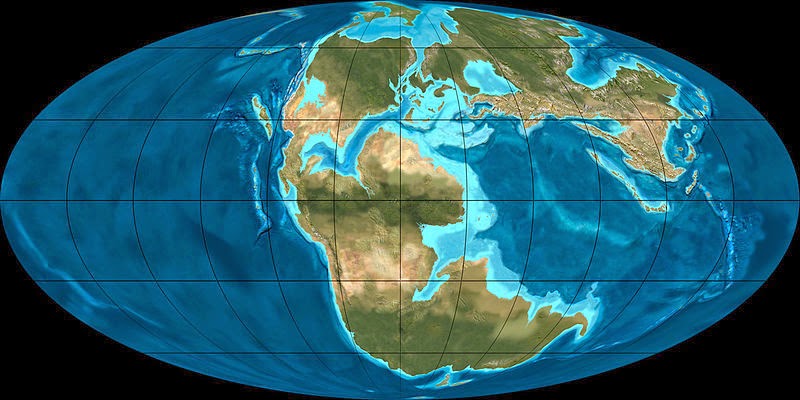
During the Late Jurassic epoch, Pangaea broke up into two supercontinents, Laurasia to the north, and Gondwana to the south. The result of this break-up was the spawning of the Atlantic Ocean. However, at this time, the Atlantic Ocean was relatively narrow.
Note : The above story is based on materials provided by Wikipedia
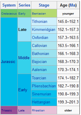
The Middle Jurassic is the second epoch of the Jurassic Period. It lasted from 176 to 161 million years ago. In European lithostratigraphy, rocks of this Middle Jurassic age are called the Dogger. This name in the past was also used to indicate the Middle Jurassic epoch itself, but is discouraged by the IUGS, to distinguish between rock units and units of geological time.
Paleogeography
During the Middle Jurassic epoch, Pangaea began to separate into Laurasia and Gondwana, and the Atlantic Ocean formed. Tectonic activities are active on eastern Laurasia as the Cimmerian plate continues to collide with Laurasia’s southern coast, completely closing the Paleo-Tethys Ocean. A subduction zone on the coast of western North America continues to create the Ancestral Rocky Mountains.
Life forms of the epoch
Marine life
During this time, marine life (including ammonites and bivalves) flourished. Ichthyosaurs, although common, are reduced in diversity; while the top marine predators, the pliosaurs, grew to the size of killer whales and larger (e.g. Pliosaurus, Liopleurodon). Plesiosaurs became common at this time, and metriorhynchid crocodilians first appeared.
Terrestrial life
New types of dinosaurs evolved on land (including cetiosaurs, brachiosaurs, megalosaurs and hypsilophodonts).
Descendants of the therapsids, the cynodonts were still flourishing along with the dinosaurs even though they were shrew-sized; none exceeded the size of a badger. A group of cynodonts, the trithelodonts were becoming rare and eventually became extinct at the end of this epoch. The Tritylodonts were still common though. Mammaliformes, who evolved from a group of cynodonts were also rare and less significant at this time. It was at this epoch that the “true” mammals evolved.
Flora
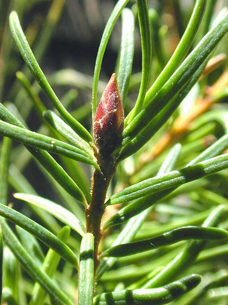
Conifers were dominant in the Middle Jurassic. Other plants, such as ginkgoes, cycads, and ferns were also common.
Note : The above story is based on materials provided by Wikipedia
The Early Jurassic epoch (in chronostratigraphy corresponding to the Lower Jurassic series) is the earliest of three epochs of the Jurassic period. The Early Jurassic starts immediately after the Triassic-Jurassic extinction event, 199.6 Ma (million years ago), and ends at the start of the Middle Jurassic (175.6 Ma).
Certain rocks of marine origin of this age in Europe are called “Lias” and that name was used for the period, as well, in 19th century geology.
Origin of the name Lias
There are two possible origins for the name Lias: the first reason is it was taken by a geologist from an English quarryman’s dialect pronunciation of the word “layers”; secondly, sloops from north Cornish ports such as Bude would sail across the Bristol Channel to the Vale of Glamorgan to load up with rock from coastal limestone quarries (lias limestone from South Wales was used throughout North Devon/North Cornwall as it contains calcium carbonate to fertilise the poor quality Devonian soils of the West Country); the Cornish would pronounce the layers of limestone as ‘laiyers’ or ‘lias’.
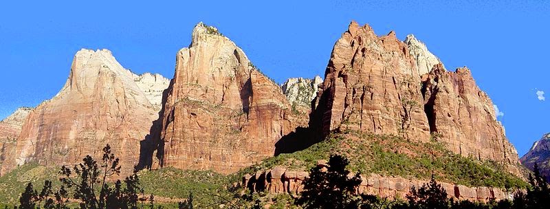
Massive cliffs in Zion Canyon consist of Lower Jurassic formations, including (from bottom to top): the Kayenta Formation and the massive Navajo Sandstone.
Geology
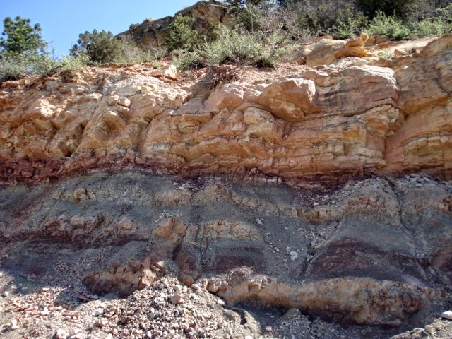
There are extensive Liassic outcrops around the coast of the United Kingdom, in particular in Glamorgan, North Yorkshire and Dorset. The ‘Jurassic Coast’ of Dorset is often associated with the pioneering work of Mary Anning of Lyme Regis. The facies of the Lower Jurassic in this area are predominantly of clays, thin limestones and siltstones, deposited under fully marine conditions.
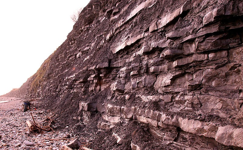
Lias Group strata form imposing cliffs on the Vale of Glamorgan coast, in southern Wales. Stretching for around 14 miles (23 km) between Cardiff and Porthcawl, the remarkable layers of these cliffs, situated on the Bristol Channel are a rhythmic decimetre scale repetition of limestone and mudstone formed as a late Triassic desert was inundated by the sea.
There has been some debate over the actual base of the Hettangian stage, and so of the Jurassic system itself. Biostratigraphically, the first appearance of psiloceratid ammonites has been used; but this depends on relatively complete ammonite faunas being present, a problem that makes correlation between sections in different parts of the world difficult. If this biostratigraphical indicator is used, then technically the Lias Group — a lithostratigraphical division — spans the Jurassic / Triassic boundary.
Life
Ammonites
During this period, ammonoids, which had almost died out at the end-of-Triassic extinction, radiated out into a huge diversity of new forms with complex suture patterns (the ammonites proper). Ammonites evolved so rapidly, and their shells are so often preserved, that they serve as important zone fossils. There were several distinct waves of ammonite evolution in Europe alone.
Marine reptiles
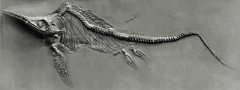
The Early Jurassic was an important time in the evolution of the marine reptiles. The Hettangian saw the already existing Rhaetian ichthyosaurs and plesiosaurs continuing to flourish, while at the same time a number of new types of these marine reptiles appeared, such as Ichthyosaurus and Temnodontosaurus among the ichthyosaurs, and Eurycleidus, Macroplata, and Rhomaleosaurus among the plesiosaurs (all Rhomaleosauridae, although as currently defined this group is probably paraphyletic). All these plesiosaurs had medium-sized necks and large heads. In the Toarcian, at the end of the Early Jurassic, the thalattosuchians (marine “crocodiles”) appeared, as did new genera of ichthyosaurs (Stenopterygius, Eurhinosaurus, and the persistently primitive Suevoleviathan) and plesiosaurs (the elasmosaurs (long-necked) Microcleidus and Occitanosaurus, and the pliosaur Hauffiosaurus).
Terrestrial animals
On land, a number of new types of dinosaurs – the heterodontosaurids, scelidosaurs, stegosaurs, and tetanurans – appeared, and joined those groups like the coelophysoids, prosauropods and the sauropods that had continued over from the Triassic. Accompanying them as small carnivores were the sphenosuchian and protosuchid crocodilians. In the air, new types of pterosaurs replaced those that had died out at the end of the Triassic. While in the undergrowth were various types of early mammals, as well as tritylodont mammal-like reptiles, lizard-like sphenodonts, and early Lissamphibians.
Note : The above story is based on materials provided by Wikipedia
The Jurassic is a geologic period and system that extends from 201.3± 0.6 Ma (million years ago) to 145± 4 Ma; from the end of the Triassic to the beginning of the Cretaceous. The Jurassic constitutes the middle period of the Mesozoic Era, also known as the Age of Reptiles. The start of the period is marked by the major Triassic–Jurassic extinction event. Two other extinction events occurred during the period: the Late Piensbachian/Early Toarcian event in the Early Jurassic, and the Late Tithonian event at the end; however, neither event ranks among the ‘Big Five’ mass extinctions. The Jurassic is named after the Jura Mountains within the European Alps, where limestone strata from the period was first identified.
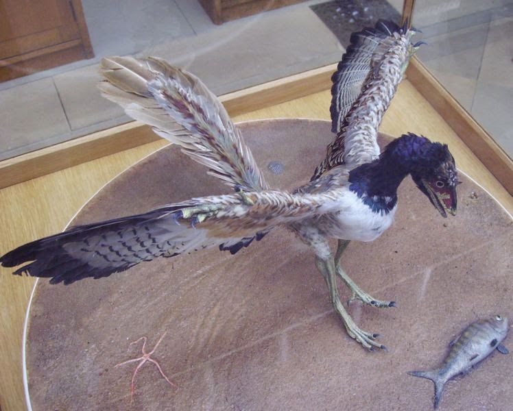
By the beginning of the Jurassic, the supercontinent Pangaea had begun rifting into two landmasses, Laurasia to the north and Gondwana to the south. This created more coastlines and shifted the continental climate from dry to humid, and many of the arid deserts of the Triassic were replaced by lush rainforests. On land, the fauna transitioned from the Triassic fauna, dominated by both dinosauromorph and crocodylomorph archosaurs, to one dominated by dinosaurs alone. The first birds also appeared during the Jurassic, having evolved from a branch of theropod dinosaurs. Other major events include the appearance of the earliest lizards, and the evolution of therian mammals, including primitive placentals. Crocodylians made the transition from a terrestrial to an aquatic mode of life. The oceans were inhabited by marine reptiles such as ichthyosaurs and plesiosaurs, while pterosaurs were the dominant flying vertebrates.
Etymology
The chronostratigraphic term “Jurassic” is directly linked to the Jura Mountains. Alexander von Humboldt recognized the mainly limestone dominated mountain range of the Jura Mountains as a separate formation that had not been included in the established stratigraphic system defined by Abraham Gottlob Werner, and he named it “Jurakalk” in 1795. The name “Jura” is derived from the Celtic root “jor”, which was Latinised into “juria”, meaning forest (i.e. “Jura” is forest mountains).
Divisions
The Jurassic period is divided into the Early Jurassic, Middle, and Late Jurassic epochs. The Jurassic System, in stratigraphy, is divided into the Lower Jurassic, Middle, and Upper Jurassic series of rock formations, also known as Lias, Dogger and Malm in Europe. The separation of the term Jurassic into three sections goes back to Leopold von Buch. The faunal stages from youngest to oldest are:
During the early Jurassic period, the supercontinent Pangaea broke up into the northern supercontinent Laurasia and the southern supercontinent Gondwana; the Gulf of Mexico opened in the new rift between North America and what is now Mexico’s Yucatan Peninsula. The Jurassic North Atlantic Ocean was relatively narrow, while the South Atlantic did not open until the following Cretaceous period, when Gondwana itself rifted apart. The Tethys Sea closed, and the Neotethys basin appeared. Climates were warm, with no evidence of glaciation. As in the Triassic, there was apparently no land near either pole, and no extensive ice caps existed.
The Jurassic geological record is good in western Europe, where extensive marine sequences indicate a time when much of the continent was submerged under shallow tropical seas; famous locales include the Jurassic Coast World Heritage Site and the renowned late Jurassic lagerstätten of Holzmaden and Solnhofen. In contrast, the North American Jurassic record is the poorest of the Mesozoic, with few outcrops at the surface. Though the epicontinental Sundance Sea left marine deposits in parts of the northern plains of the United States and Canada during the late Jurassic, most exposed sediments from this period are continental, such as the alluvial deposits of the Morrison Formation.
The Jurassic was a time of calcite sea geochemistry in which low-magnesium calcite was the primary inorganic marine precipitate of calcium carbonate. Carbonate hardgrounds were thus very common, along with calcitic ooids, calcitic cements, and invertebrate faunas with dominantly calcitic skeletons (Stanley and Hardie, 1998, 1999).
The first of several massive batholiths were emplaced in the northern Cordillera beginning in the mid-Jurassic, marking the Nevadan orogeny. Important Jurassic exposures are also found in Russia, India, South America, Japan, Australasia and the United Kingdom.
The late Jurassic Morrison Formation in Colorado is one of the most fertile sources of dinosaur fossils in North America.
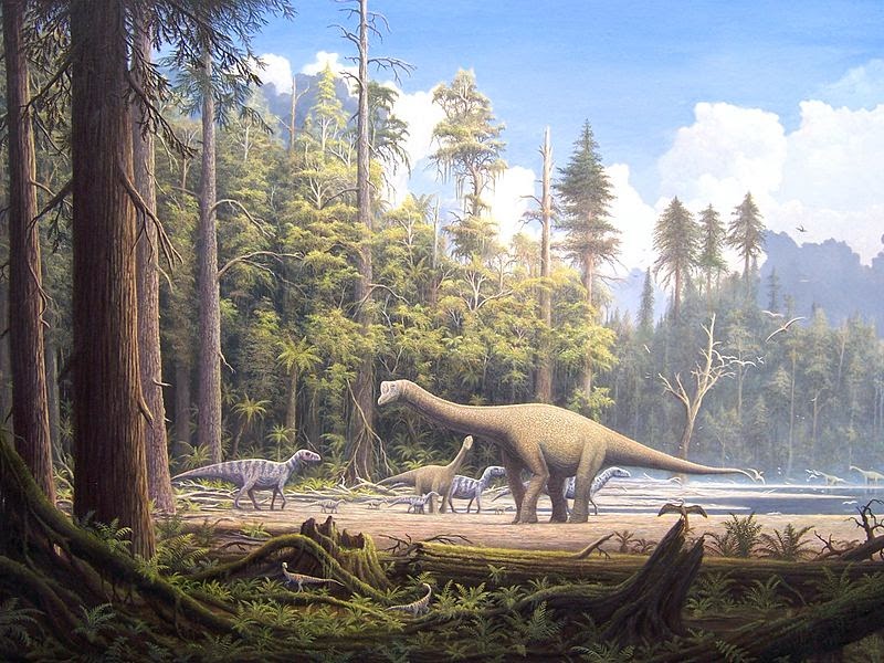
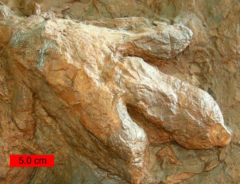
In Africa, Early Jurassic strata are distributed in a similar fashion to Late Triassic beds, with more common outcrops in the south and less common fossil beds which are predominated by tracks to the north. As the Jurassic proceeded, larger and more iconic groups of dinosaurs like sauropods and ornithopods proliferated in Africa. Middle Jurassic strata are neither well represented nor well studied in Africa. Late Jurassic strata are also poorly represented apart from the spectacular Tendeguru fauna in Tanzania. The Late Jurassic life of Tendeguru is very similar to that found in western North America’s Morrison Formation.
Fauna
Aquatic and marine
During the Jurassic period, the primary vertebrates living in the sea were fish and marine reptiles. The latter include ichthyosaurs, who were at the peak of their diversity, plesiosaurs, pliosaurs, and marine crocodiles of the families Teleosauridae and Metriorhynchidae. Numerous turtles could be found in lakes and rivers.
In the invertebrate world, several new groups appeared, including rudists (a reef-forming variety of bivalves) and belemnites. Calcareous sabellids (Glomerula) appeared in the Early Jurassic. The Jurassic also had diverse encrusting and boring (sclerobiont) communities, and it saw a significant rise in the bioerosion of carbonate shells and hardgrounds. Especially common is the ichnogenus (trace fossil) Gastrochaenolites.
During the Jurassic period, about four or five of the twelve clades of planktonic organisms that exist in the fossil record either experienced a massive evolutionary radiation or appeared for the first time.
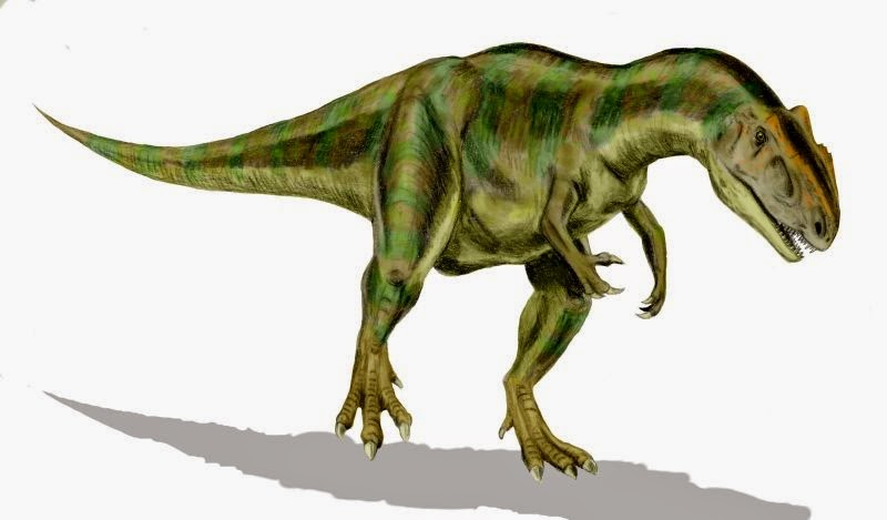
On land, large archosaurian reptiles remained dominant. The Jurassic was a golden age for the large herbivorous dinosaurs known as the sauropods—Camarasaurus, Apatosaurus, Diplodocus, Brachiosaurus, and many others—that roamed the land late in the period; their mainstays were either the prairies of ferns, palm-like cycads and bennettitales, or the higher coniferous growth, according to their adaptations. They
were preyed upon by large theropods, such as Ceratosaurus, Megalosaurus, Torvosaurus and Allosaurus. All these belong to the ‘lizard hipped’ or saurischian branch of the dinosaurs. During the Late Jurassic, the first Avialans, like Archaeopteryx, evolved from small coelurosaurian dinosaurs. Ornithischian dinosaurs were less predominant than saurischian dinosaurs, although some, like stegosaurs and small ornithopods, played important roles as small and medium-to-large (but not sauropod-sized) herbivores. In the air, pterosaurs were common; they ruled the skies, filling many ecological roles now taken by birds. Within the undergrowth were various types of early mammals, as well as tritylodonts, lizard-like sphenodonts, and early lissamphibians.
The rest of the Lissamphibia evolved in this period, introducing the first salamanders and caecilians.
The arid, continental conditions characteristic of the Triassic steadily eased during the Jurassic period, especially at higher latitudes; the warm, humid climate allowed lush jungles to cover much of the landscape. Gymnosperms were relatively diverse during the Jurassic period. The Conifers in particular dominated the flora, as during the Triassic; they were the most diverse group and constituted the majority of large trees.
Extant conifer families that flourished during the Jurassic included the Araucariaceae, Cephalotaxaceae, Pinaceae, Podocarpaceae, Taxaceae and Taxodiaceae. The extinct Mesozoic conifer family Cheirolepidiaceae dominated low latitude vegetation, as did the shrubby Bennettitales. Cycads were also common, as were ginkgos and Dicksoniaceous tree ferns in the forest. Smaller ferns were probably the dominant undergrowth. Caytoniaceous seed ferns were another group of important plants during this time and are thought to have been shrub to small-tree sized. Ginkgo plants were particularly common in the mid- to high northern latitudes. In the Southern Hemisphere, podocarps were especially successful, while Ginkgos and Czekanowskiales were rare.
In the oceans, modern coralline algae appeared for the first time.
Note : The above story is based on materials provided by Wikipedia
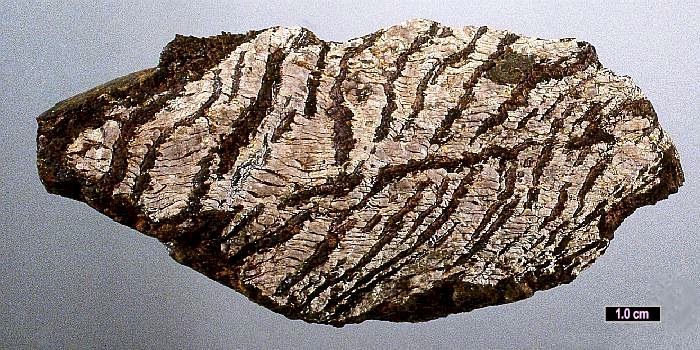
Chemical Formula: Pb9As4S15 Locality: In the Excelsior mine, Cerro de Pasco, Peru, in large crystals. Name Origin: For Louis Carly Graton (1880-1970), Professor of Economic Geology, Harvard University, Cambridge, Massachusetts, USA.
Gratonite is a lead-arsenic sulfosalt mineral, with the chemical composition Pb9As4S15. Gratonite was discovered in 1939 at the Excelsior Mine, Cerro de Pasco, Peru. It is named in honor of geologist L. C. Graton (1880–1970), who had a long-standing association with the Cerro de Pasco mines.
Physical Properties
Cleavage: None Color: Lead gray, Dark lead gray. Density: 6.22 Diaphaneity: Opaque Fracture: Brittle – Generally displayed by glasses and most non-metallic minerals. Hardness: 2.5 – Finger Nail Luster: Metallic Streak: black
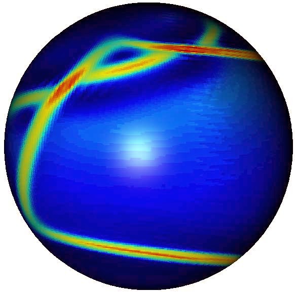
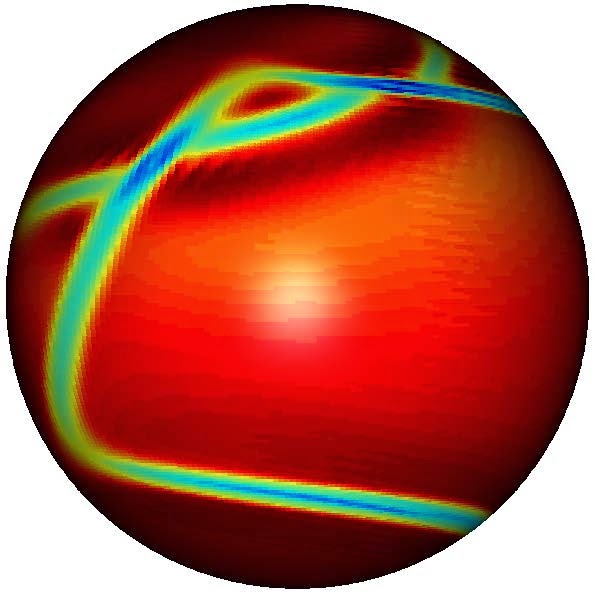
An idealized simulation showing how plate-tectonic boundaries (including complex ones) emerge because of inherited damage following a shift in plate-tectonic driving forces; in this case the shift is similar to that which caused the Emperor-Hawaiian Bend in the Pacific. Credit: David Bercovici
(Phys-org) —Two researchers, David Bercovici of Yale University and Yanick Ricard with the University of Lyon, have together used mathematical modeling to help explain how it was that our planet came to have tectonic plates and why they behave the way they do today. In their paper published in the journal Nature, the pair have explained how they performed mathematical analysis on observations of rocks today and combined data taken from prior theories to come up with a new model that might reflect Earth’s history during the first billion years of its existence.
The surface of planet Earth is covered in several moving plates which scientists believe is one of the major reasons that life was able to evolve and survive. But how the plates came to exist and wound up behaving the way they do today, has been mostly a mystery. In this new effort, the model built by the researchers offers one possible explanation.
It all comes down to grains of rock, they suggest—the smaller the grain, the weaker the rock. One type of rock, known as mylonite has been found to exist at every plate boundary on the planet, suggesting it has something to do with plate tectonics—when found, it is generally deformed with very small grains.
Bercovici and Ricard’s model starts with the idea that very early Earth was covered in hot mushy material. As that material began to cool, some parts or regions would cool faster or slower than others—the cooler parts would then naturally sink. Prior studies have shown that when such types of material sink, the surface becomes slightly deformed. With rock, scientists already known that deformations lead to weaker rock and subsequently smaller grains—and weaker rock would of course lead to additional deformations which suggests a feed-back loop would have evolved. On a planet-wide scale that would mean that weak zones would form at boundaries giving rise to the evolution of tectonic plates. Over billions of years, as the planet continued cooling, the result would be plate tectonics.
The same model can be used to explain why other planets in our solar system didn’t develop plates, and thus the conditions necessary for the development of life. Venus, for example, the numbers suggest, was simply too hot. If pre-plates developed, the deformations would heal due to the high temperatures, preventing the development of actual plates and possibly an atmosphere conducive to life.
An idealized simulation showing how plate-tectonic boundaries (including complex ones) emerge because of inherited damage following a shift in plate-tectonic driving forces; in this case the shift is similar to that which caused the Emperor-Hawaiian Bend in the Pacific. Credit: David Bercovici
Abstract:
The initiation of plate tectonics on Earth is a critical event in our planet’s history. The time lag between the first proto-subduction (about 4 billion years ago) and global tectonics (approximately 3 billion years ago) suggests that plates and plate boundaries became widespread over a period of 1 billion years. The reason for this time lag is unknown but fundamental to understanding the origin of plate tectonics. Here we suggest that when sufficient lithospheric damage (which promotes shear localization and long-lived weak zones) combines with transient mantle flow and migrating proto-subduction, it leads to the accumulation of weak plate boundaries and eventually to fully formed tectonic plates driven by subduction alone. We simulate this process using a grain evolution and damage mechanism with a composite rheology (which is compatible with field and laboratory observations of polycrystalline rocks1, 2), coupled to an idealized model of pressure-driven lithospheric flow in which a low-pressure zone is equivalent to the suction of convective downwellings. In the simplest case, for Earth-like conditions, a few successive rotations of the driving pressure field yield relic damaged weak zones that are inherited by the lithospheric flow to form a nearly perfect plate, with passive spreading and strike-slip margins that persist and localize further, even though flow is driven only by subduction. But for hotter surface conditions, such as those on Venus, accumulation and inheritance of damage is negligible; hence only subduction zones survive and plate tectonics does not spread, which corresponds to observations. After plates have developed, continued changes in driving forces, combined with inherited damage and weak zones, promote increased tectonic complexity, such as oblique subduction, strike-slip boundaries that are subparallel to plate motion, and spalling of minor plates.
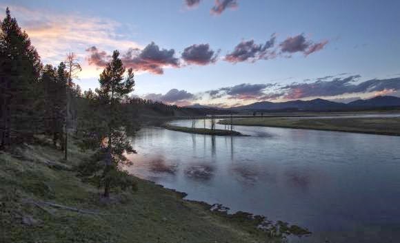
The Yellowstone River winds through the Hayden Valley in Yellowstone National Park, Wyoming, June 9, 2013. Credit: Reuters/Jim Urquhart
(Reuters) – Yellowstone National Park assured guests and the public on Thursday that a super-volcano under the park was not expected to erupt anytime soon, despite an alarmist video that claimed bison had been seen fleeing to avoid such a calamity.
Yellowstone officials, who fielded dozens of calls and emails since the video went viral this week following an earthquake in the park, said the video actually shows bison galloping down a paved road that leads deeper into the park.
“It was a spring-like day and they were frisky. Contrary to online reports, it’s a natural occurrence and not the end of the world,” park spokeswoman Amy Bartlett said.
Assurances by Yellowstone officials and government geologists that the ancient super-volcano beneath the park is not due to explode for eons have apparently done little to quell fears among the thousands who have viewed recent video postings of the thundering herd.
Commentary with one of the clips by a self-described survivalist wearing camouflage, dark sunglasses and a black watch cap suggests the wildlife exodus may be tied to “an imminent eruption here at Yellowstone.”
The 4.8 magnitude earthquake that struck early Sunday near the Norris Geyser Basin in the northwest section of Yellowstone, which spans 3,472 square miles of Wyoming, Montana and Idaho, caused no injuries or damages and did not make any noticeable alterations to the landscape, geologists said.
Though benign by seismic standards, it was the largest to rattle Yellowstone since a 4.8 quake in February 1980 and it occurred near an area of ground uplift tied to the upward movement of molten rock in the super-volcano, whose mouth, or caldera, is 50 miles long and 30 miles wide.
But neither the quake, the largest among hundreds that have struck near the geyser basin in the last seven months, nor the uplift suggest an eruption sooner than tens of thousands of years, said Peter Cervelli, associate director for science and technology at the U.S. Geological Survey’s Volcano Science Center in California.
“The chance of that happening in our lifetimes is exceedingly insignificant,” said Cervelli, a scientist with the Yellowstone Volcano Observatory.
Cervelli said the area of uplift that scientists have been tracking since August is rising at a rate of between 10 centimeters (4 inches) and 15 centimeters a year. Geologists who tracked uplift in the same area from 1996 to 2003 also saw elevated seismic activity, he said.
Video :
Note : Note : The above story is based on materials provided by Dan Whitcomb and Steve Orlofsky to Reuters
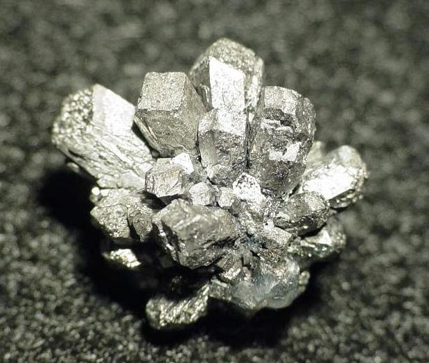
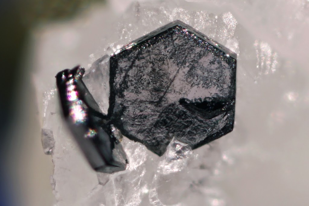
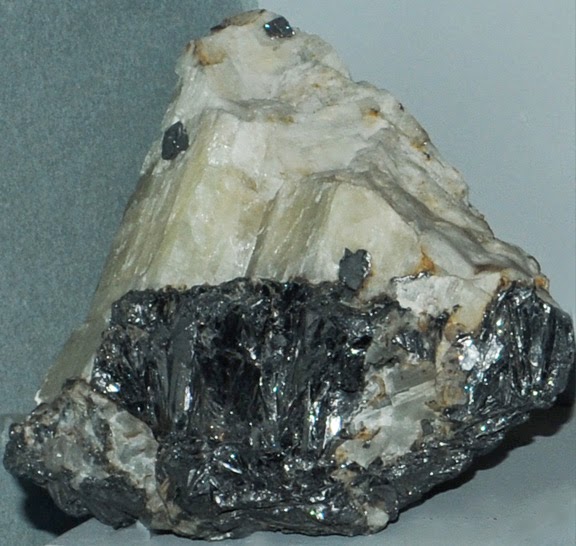
Chemical Formula: C Locality: Ticonderoga, New York. Madagascar and Ceylon. Name Origin: From the Greek, graphein, “to write.”
Graphite is made almost entirely of carbon atoms, and as with diamond, is a semimetal native element mineral, and an allotrope of carbon. Graphite is the most stable form of carbon under standard conditions. Therefore, it is used in thermochemistry as the standard state for defining the heat of formation of carbon compounds. Graphite may be considered the highest grade of coal, just above anthracite and alternatively called meta-anthracite, although it is not normally used as fuel because it is difficult to ignite.
Occurrence
Graphite occurs in metamorphic rocks as a result of the reduction of sedimentary carbon compounds during metamorphism. It also occurs in igneous rocks and in meteorites. Minerals associated with graphite include quartz, calcite, micas and tourmaline. In meteorites it occurs with troilite and silicate minerals. Small graphitic crystals in meteoritic iron are called cliftonite.
According to the United States Geological Survey (USGS), world production of natural graphite in 2012 was 1,100,000 tonnes, of which the following major exporters are: China (750 kt), India (150 kt), Brazil (75 kt), North Korea (30 kt) and Canada (26 kt). Graphite is not mined in the United States, but U.S. production of synthetic graphite in 2010 was 134 kt valued at $1.07 billion.
Physical Properties
Cleavage: {0001} Perfect Color: Iron black, Dark gray, Black, Steel gray. Density: 2.09 – 2.23, Average = 2.16 Diaphaneity: Opaque Fracture: Sectile – Curved shavings or scrapings produced by a knife blade, (e.g. graphite). Hardness: 1.5-2 – Talc-Gypsum Luminescence: Non-fluorescent. Luster: Sub Metallic Magnetism: Nonmagnetic Streak: black
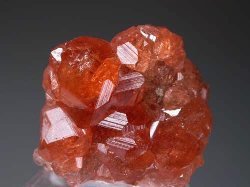
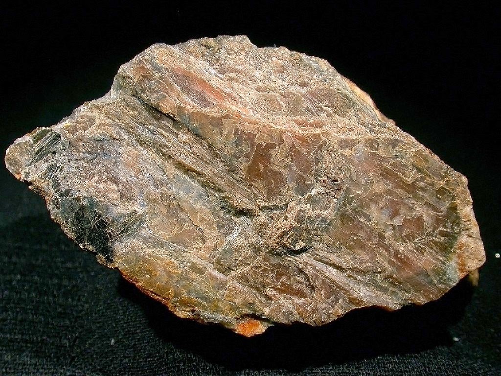
Chemical Formula: (Fe2+,Mn,Ca)3(PO4)2 Name Origin: Named after its locality at Grafton, New Hampshire, USA.
Graftonite is an iron(II), manganese, calcium phosphate mineral with formula: (Fe2+,Mn,Ca)3(PO4)2. It forms lamellar to granular translucent brown to red-brown to pink monoclinic prismatic crystals. It has a vitreous luster with a Mohs hardness of 5 and a specific gravity of 3.67 to 3.7.
It was first described from its type locality of Melvin Mountain in the town of Grafton, in Grafton County, New Hampshire.
Physical Properties
Cleavage: {010} Perfect Color: Brown, Pink, Dark brown, Reddish brown. Density: 3.67 – 3.7, Average = 3.68 Diaphaneity: Translucent Fracture: Uneven – Flat surfaces (not cleavage) fractured in an uneven pattern. Hardness: 5 – Apatite Luminescence: Non-fluorescent. Luster: Vitreous – Greasy Streak: pale pink
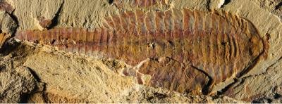
This image shows the dorsal view of Fuxianhuia protensa. The three-inch-long fossil was found in sediments dating from the Cambrian Period 520 million years ago in what today is the Yunnan province in China. Parts of the gut are visible as dark stains along the animal’s midline. Credit: Xiaoya Ma
In 520 million-year-old fossil deposits resembling an ‘invertebrate version of Pompeii,’ researchers have found an ancestor of modern crustaceans revealing the first-known cardiovascular system in exquisitely preserved detail
An international team of researchers from the University of Arizona, China and the United Kingdom has discovered the earliest known cardiovascular system, and the first to clearly show a sophisticated system complete with heart and blood vessels, in fossilized remains of an extinct marine creature that lived over half a billion years ago. The finding sheds new light on the evolution of body organization in the animal kingdom and shows that even the earliest creatures had internal organizational systems that strongly resemble those found in their modern descendants.
“This is the first preserved vascular system that we know of,” said Nicholas Strausfeld, a Regents’ Professor of Neuroscience at the University of Arizona’s Department of Neuroscience, who helped analyze the find.
Being one of the world’s foremost experts in arthropod morphology and neuroanatomy, Strausfeld is no stranger to finding meaningful and unexpected answers to long-standing mysteries in the remains of creatures that went extinct so long ago scientists still argue over where to place them in the evolutionary tree.
The 3-inch-long fossil was entombed in fine dustlike particles – now preserved as fine-grain mudstone – during the Cambrian Period 520 million years ago in what today is the Yunnan province in China. Found by co-author Peiyun Cong near Kunming, it belongs to the species Fuxianhuia protensa, an extinct lineage of arthropods combining advanced internal anatomy with a primitive body plan.
“Fuxianhuia is relatively abundant, but only extremely few specimens provide evidence of even a small part of an organ system, not even to speak of an entire organ system,” said Strausfeld, who directs the UA Center for Insect Science. “The animal looks simple, but its internal organization is quite elaborate. For example, the brain received many arteries, a pattern that appears very much like a modern crustacean.”
In fact, Strausfeld pointed out, Fuxianhuia’s vascular system is more complex than what is found in many modern crustaceans.
“It appears to be the ground pattern from which others have evolved,” he said. “Different groups of crustaceans have vascular systems that have evolved into a variety of arrangements but they all refer back to what we see in Fuxianhuia.”
“Over the course of evolution, certain segments of the animals’ body became specialized for certain things, while others became less important and, correspondingly, certain parts of the vascular system became less elaborate,” Strausfeld said.
Strausfeld helped identify the oldest known fossilized brain in a different specimen of the same fossil species, as well as the first evidence of a completely preserved nervous system similar to that of a modern chelicerates, such as a horseshoe crab or a scorpion.
“This is another remarkable example of the preservation of an organ system that nobody would have thought could become fossilized,” he said.
In addition to the exquisitely preserved heart and blood vessels, outlined as traces of carbon embedded in the surrounding mineralized remains of the fossil, it also features the eyes, antennae and external morphology of the animal.
Using a clever imaging technique that selectively reveals different structures in the fossil based on their chemical composition, collaborator Xiaoya Ma at London’s Natural History Museum was able to identify the heart, which extended along the main part of the body, and its many lateral arteries corresponding to each segment. Its arteries were composed of carbon-rich deposits and gave rise to long channels, which presumably took blood to limbs and other organs.
“With that, we can now start speculating about behavior,” Strausfeld explained. “Because of well-supplied blood vessels to its brain, we can assume this was a very active animal capable of making many different behavioral choices.”
Researchers can only speculate as to why the chemical reactions that occurred during the process of fossilization allowed for this unusual and rare kind of preservation, and as to why only select tissues were preserved between a few rare and different specimen.
“Presumably the conditions had to be just right,” Strausfeld said. “We believe that these animals were preserved because they were entombed quickly under very fine-grained deposits during some kind of catastrophic event, and were then permeated by certain chemicals in the water while they were squashed flat. It is an invertebrate version of Pompeii.”
Possibly, only one in thousands of fossils might have such a well-preserved organ system, Strausfeld said.
At the time Fuxianhuia crawled on the seafloor or swam through water, life had not yet conquered land.
“Terrible sand storms must have occurred because there were probably no plants that could hold the soils,” Strausfeld said. “The habitats of these creatures must have been inundated with massive fallouts from huge storms.”
Tsunamis may also be the cause for the exceptional preservation.
“As the water withdraws, animals on the seafloor dry,” Strausfeld said. “When the water rushed back in, they might become inundated with mud. Under normal circumstances, when animals die and are left to rot on the seafloor, they become unrecognizable. What happened to provide the kinds of fossils we are seeing must have been very different.”
Note : Note : The above story is based on materials provided by University of Arizona
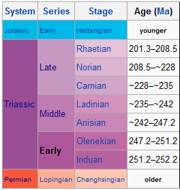
The Early Triassic is the first of three epochs of the Triassic Period of the geologic timescale. It spans the time between 252.2 ± 0.5 Ma and 247.2 Ma (million years ago). Rocks from this epoch are collectively known as the Lower Triassic, which is a unit in chronostratigraphy. The Early Triassic is the oldest epoch of the Mesozoic Era and is divided into the Induan and Olenekian ages.
The Lower Triassic series is coeval with the Scythian stage, which is today not included in the official timescales but can be found in older literature. In Europe, most of the Lower Triassic is composed of Buntsandstein, a lithostratigraphic unit of continental red beds.
The Permian-Triassic extinction event spawned the Triassic period. The massive extinctions that ended the Permian period and Paleozoic era caused extreme hardships for the surviving species. Many types of corals, brachiopods, molluscs, echinoderms, and other invertebrates had completely disappeared. The most common Early Triassic hard-shelled marine invertebrates were bivalves, gastropods, ammonites, echinoids, and a few articulate brachiopods. The most common land animal was the small herbivorous synapsid Lystrosaurus.
Early Triassic faunas lacked biodiversity and were relatively homogenous throughout the epoch due to the effects of the extinction, ecological recovery on land took 30M years. The climate during the Early Triassic epoch (especially in the interior of the supercontinent Pangaea) was generally arid, rainless and dry and deserts were widespread however the poles possessed a temperate climate. The relatively hot climate of the Early Triassic may have been caused by widespread volcanic eruptions which accelerated the rate of global warming and possibly caused the Permian Triassic extinction event.
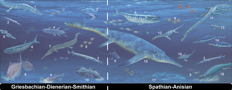
Smithian-Spathian extinction
Until recently the existence of an extinction event about 3 million years following the end-Permian extinctions was not recognised, possibly because there were few species left to go extinct. However, studies on conodonts have revealed that temperatures rose in the first 3 million years of the Triassic, ultimately reaching sea surface temperatures of 40 °C in the tropics around 249 million years ago. Large and mobile species disappeared from the tropics, and amongst the immobile species such as molluscs only the ones that could cope with the heat survived; half the bivalves disappeared. On land the tropics were practically devoid of life.
Big, active animals only returned to the tropics, and plants recolonised on land when temperatures returned to normal around 247 million years ago.
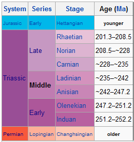
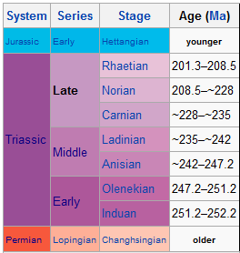
Subdivision of the Triassic system according to the IUGS, as of July 2012.
In the geologic timescale, the Middle Triassic is the second of three epochs of the Triassic period or the middle of three series in which the Triassic system is divided. It spans the time between 247.2 Ma and ~235 Ma (million years ago). The Middle Triassic is divided into the Anisian and Ladinian ages or stages.
Formerly the middle series in the Triassic was also known as Muschelkalk. This name is now only used for a specific unit of rock strata with approximately Middle Triassic age, found in western Europe.
During this time there were no flowering plants, but instead there were ferns and mosses. Small dinosaurs began to appear like Nyasasaurus.
Note : The above story is based on materials provided by Wikipedia
Subdivision of the Triassic systemaccording to the IUGS, as of July 2012.
The Late Triassic is in the geologic timescale the third and final of three epochs of the Triassic period. The corresponding series is known as the Upper Triassic. In the past it was sometimes called the Keuper, after a German lithostratigraphic group (a sequence of rock strata) that has a roughly corresponding age. The Late Triassic spans the time between ~235 Ma and 201.3 ± 0.2 Ma (million years ago). The Late Triassic is divided into the Carnian, Norian and Rhaetian ages.
Many of the first dinosaurs evolved during the Late Triassic, including Plateosaurus, Coelophysis, and Eoraptor.
Paleogeography and tectonics
Africa shared Pangea’s relatively uniform fauna which was dominated by theropods, prosauropods and primitive ornithischians by the close of the Triassic period. Late Triassic fossils are found throughout Africa, but are more common in the south than north.
The boundary separating the Triassic and Jurassic marks the advent of an extinction event with global impact, although African strata from this time period have not been thoroughly studied. In the area of Tübingen (Germany), a Triassic-Jurassic bonebed can be found, which is characteristic for this boundary.
Note : The above story is based on materials provided by Wikipedia