Researchers have developed a new approach to simulating the energetic processes that may have led to the emergence of cell metabolism on Earth — a crucial biological function for all living organisms.
The research, which is published online today in the journal Astrobiology, could help scientists to understand whether it is possible for life to have emerged in similar environments on other worlds.
Dr Terry Kee from the School of Chemistry at the University of Leeds, one of the co-authors of the research paper, said: “What we are trying to do is to bridge the gap between the geological processes of the early Earth and the emergence of biological life on this planet.”
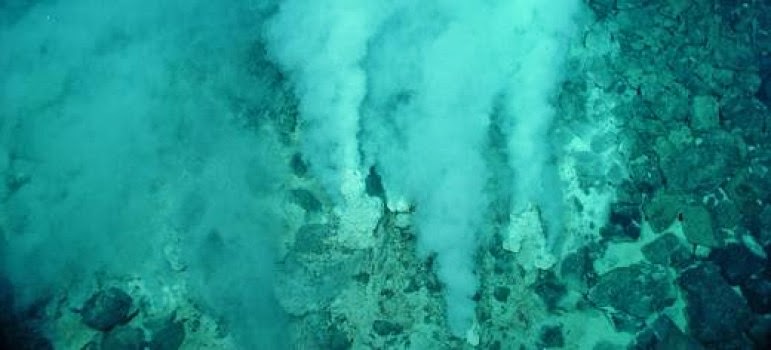
Previously, some scientists have proposed that living organisms may have been transported to Earth by meteorites. Yet there is more support for the theory that life emerged on Earth in places like hydrothermal vents on the ocean floor, forming from inanimate matter such as the chemical compounds found in gases and minerals.
“Before biological life, one could say the early Earth had ‘geological life’. It may seem unusual to consider geology, involving inanimate rocks and minerals, as being alive. But what is life?” said Dr Kee.
“Many people have failed to come up with a satisfactory answer to this question. So what we have done instead is to look at what life does, and all life forms use the same chemical processes that occur in a fuel cell to generate their energy.”
Fuel cells in cars generate electrical energy by reacting fuels and oxidants. This is an example of a ‘redox reaction’, as one molecule loses electrons (is oxidised) and one molecule gains electrons (is reduced).
Similarly, photosynthesis in plants involves generating electrical energy from the reduction of carbon dioxide into sugars and the oxidation of water into molecular oxygen. And respiration in cells in the human body is the oxidation of sugars into carbon dioxide and the reduction of oxygen into water, with electrical energy produced in the reaction.
Certain geological environments, such as hydrothermal vents can be considered as ‘environmental fuel cells’, since electrical energy can be generated from redox reactions between hydrothermal fuels and seawater oxidants, such as oxygen. Indeed, last year researchers in Japan demonstrated that electrical power can be harnessed from these vents in a deep-sea experiment in Okinawa.
In the new study, the researchers have demonstrated a proof of concept for their fuel cell model of the emergence of cell metabolism on Earth.
In the Energy Leeds Renewable Lab at the University of Leeds and NASA’s Jet Propulsion Laboratory, the team replaced traditional platinum catalysts in fuel cells and electrical experiments with those composed of geological minerals.
Dr Laura Barge from the NASA Astrobiology Institute ‘Icy Worlds’ team at JPL in California, US, and lead author of the paper, said: “Certain minerals could have driven geological redox reactions, later leading to a biological metabolism. We’re particularly interested in electrically conductive minerals containing iron and nickel that would have been common on the early Earth.”
Iron and nickel are much less reactive than platinum. However, a small but significant power output successfully demonstrated that these metals could still generate electricity in the fuel cell — and hence also act as catalysts for redox reactions within hydrothermal vents in the early Earth.
For now, the chemistry of how geological reactions driven by inanimate rocks and minerals evolved into biological metabolisms is still a black box. But with a laboratory-based model for simulating these processes, scientists have taken an important step forward to understanding the origin of life on this planet and whether a similar process could occur on other worlds.
Dr Barge said: “These experiments simulate the electrical energy produced in geological systems, so we can also use this to simulate other planetary environments with liquid water, like Jupiter’s moon Europa or early Mars.
“With these techniques we could actually test whether any given hydrothermal system could produce enough energy to start life, or even, provide energetic habitats where life might still exist and could be detected by future missions.”
Video :
Note : The above story is based on materials provided by University of Leeds.
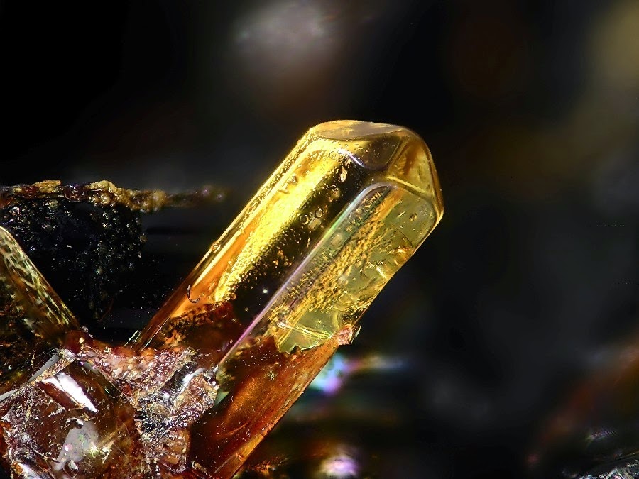
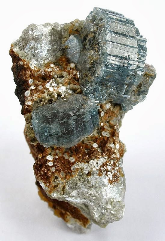
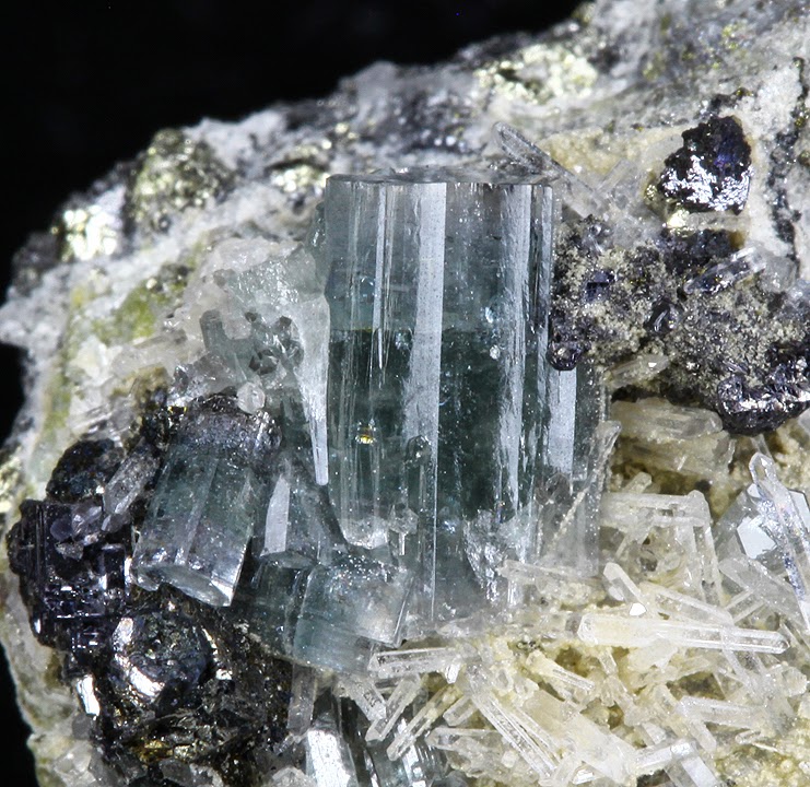
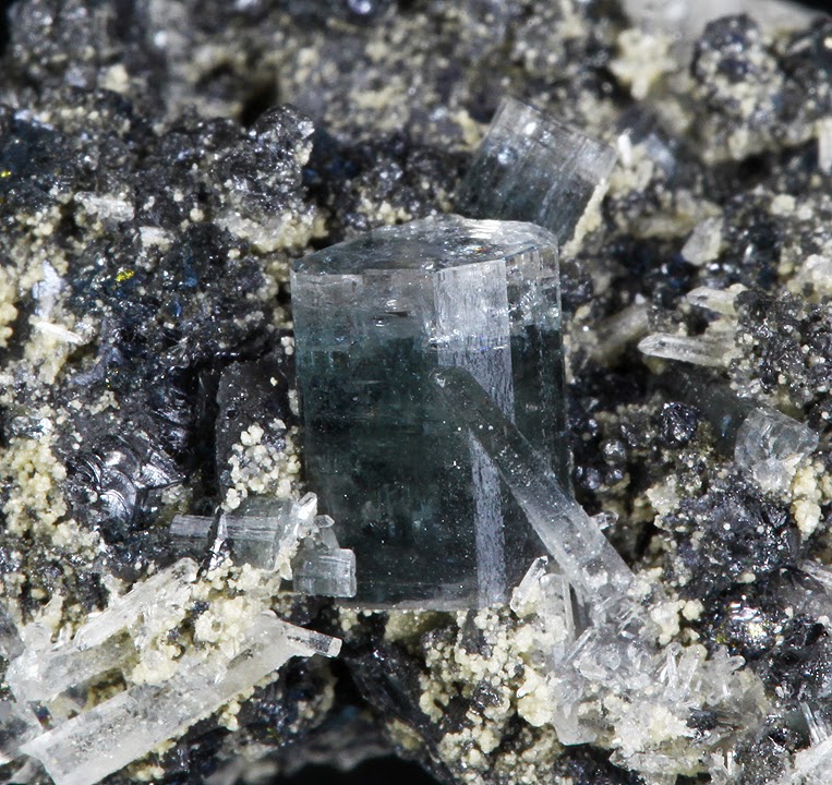
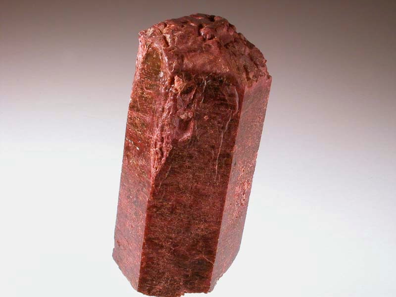
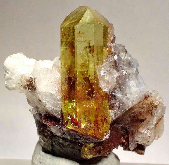


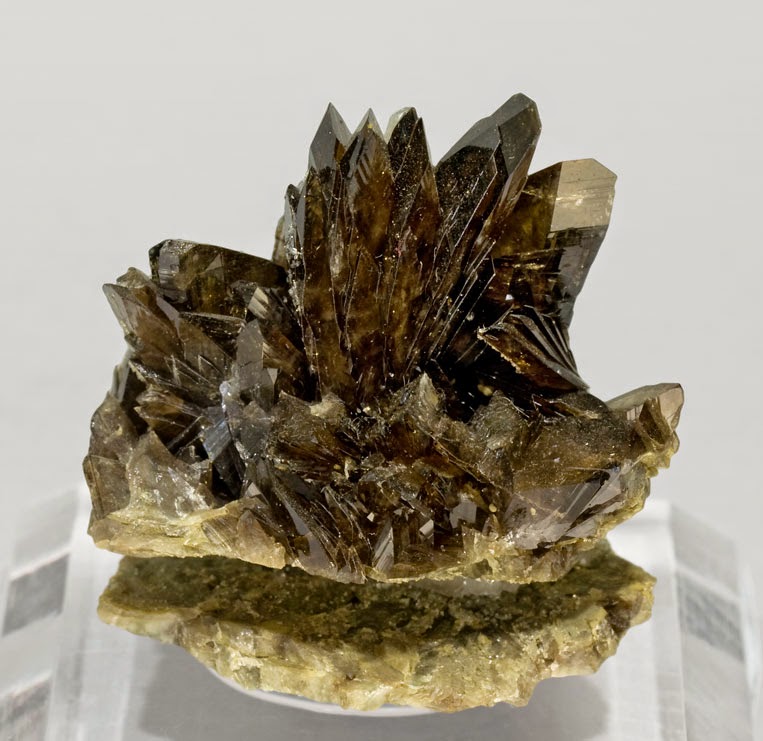
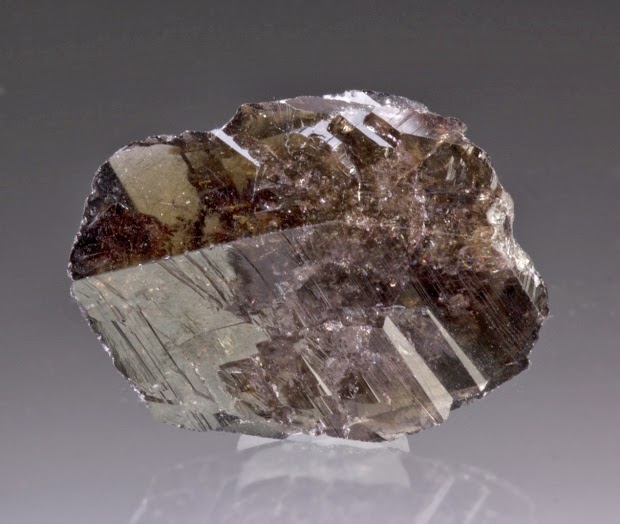
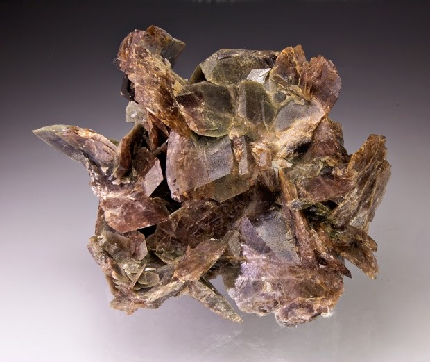
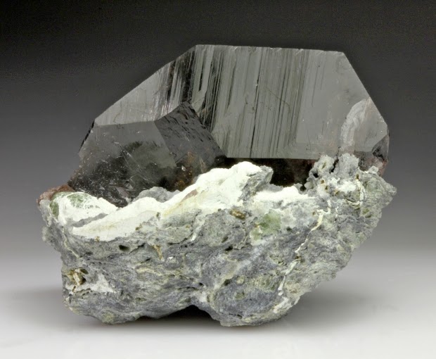
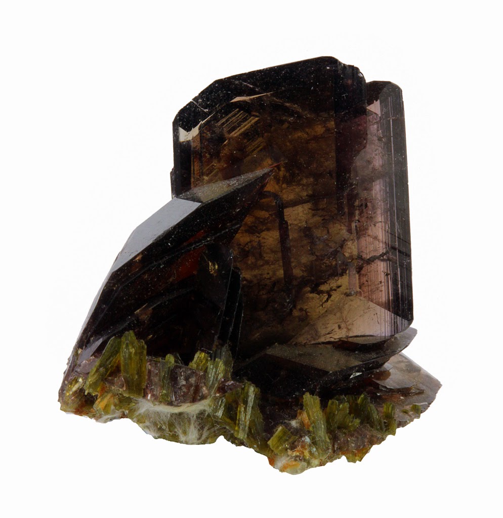

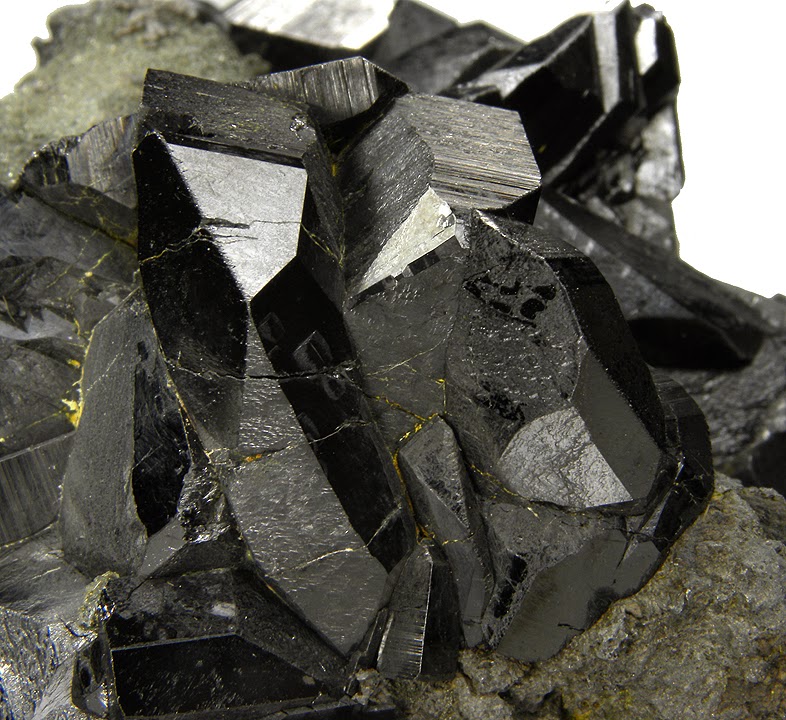
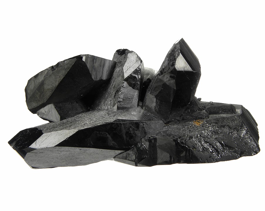
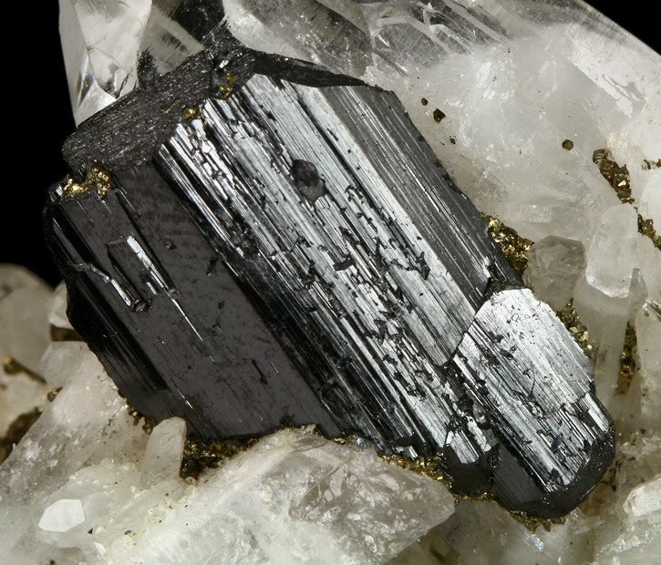
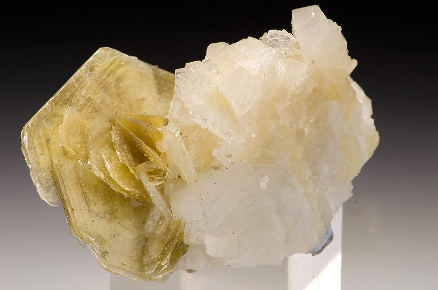
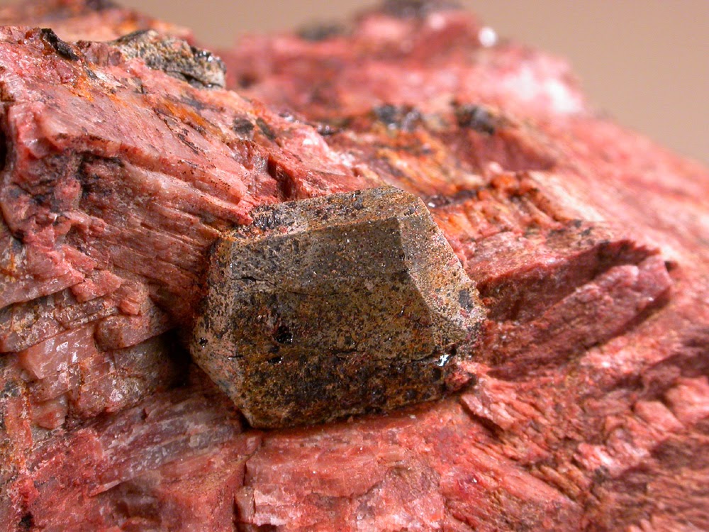
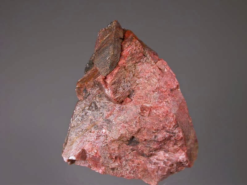
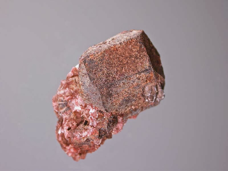
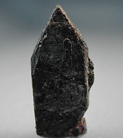
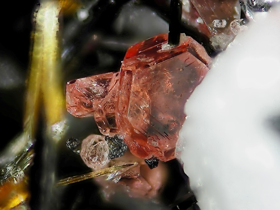
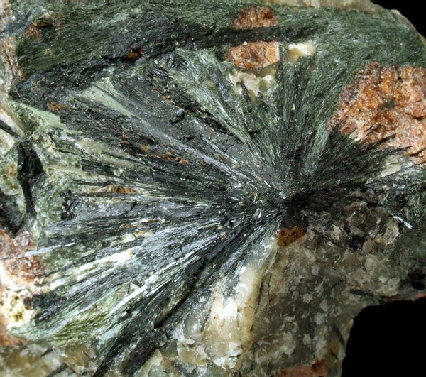
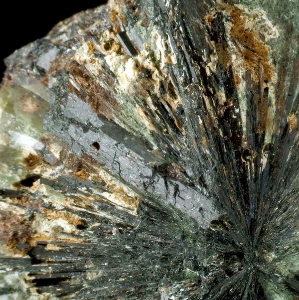
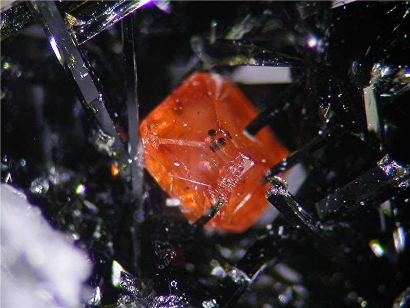
 Chemical Formula: FeWO4