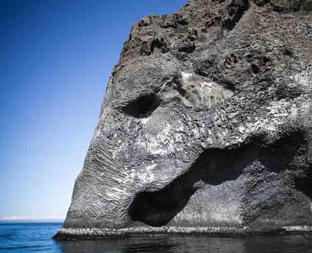
A bleached fringe of dead marine algae, strung along the coastlines of two islands off the coast of Chile, offers a unique glimpse at how the land rose during the 2016 magnitude 7.6 Chiloé earthquake, according to a new study in the Bulletin of the Seismological Society of America.
Durham University researcher Ed Garrett and colleagues used the algal data to help confirm the amount of fault slip that occurred during the Chiloé quake, which took place in an area that had been seismically quiet since the 1960 magnitude 9.5 Valdivia earthquake—the largest instrumentally recorded earthquake in the world.
There are fewer records of more moderate earthquakes in the region, so “precisely quantifying the amount and distribution of slip in 2016 therefore helps us to understand the characteristics of these smaller events. This information helps us to better assess how faults accumulate and release strain during sequences of ruptures of different magnitudes,” said Garrett.
“Such insights in turn assist with efforts to assess future seismic hazards,” he added. “While the 2016 earthquake occurred in a sparsely populated region, similar major earthquakes on the Chilean Subduction Zone could pose significant hazards to more populous regions in the future.”
Garrett and colleagues combined their calculations of the amount of uplift indicated by the algal data—about 25.8 centimeters—with satellite data of the crust’s movement during the earthquake to determine that the maximum slip along the fault was approximately three meters.
The slip is equivalent to about 80 percent of the maximum cumulative plate convergence since the 1960 Valdivia earthquake, they conclude, which is a result similar to other recent estimates of slip. Some of the earliest reports from the 2016 earthquake suggested that the maximum fault slip during the event was as much as five meters, which would have wiped out or exceeded all the seismic stress built up by plate convergence since the 1960 earthquake.
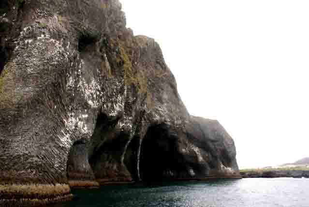
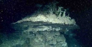
When an earthquake rupture lifts coastal crust, it can strand organisms like algae and mussels that fix themselves to rocks, raising their homes above their normal waterline. The catastrophe leaves a distinctive line of dead organisms traced across the rock. The distance between the upper limit of this death zone and the upper limit of the zone containing living organisms offers an estimate of the vertical uplift of the crust.
Researchers have long used the technique to measure abrupt vertical deformation of the crust. During the famous 19th century voyage of the HMS Beagle, Charles Darwin used a band of dead mussels to determine the uplift of Isla Santa María during the magnitude 8.5 Chilean earthquake of 1835.
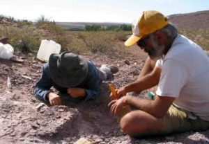
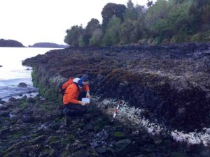
Ten months after the Chiloé earthquake, Garrett and his colleagues were studying the effects of the quake on coastal environments such as tidal marshes, looking for modern examples of how earthquakes affect these environments that they could use in their study of prehistoric earthquakes.
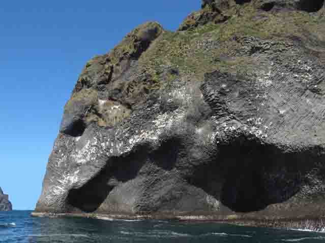
“It was only once we reached Isla Quilán that we noticed the band of bleached coralline algae along the rocky shorelines and realized that we could use this marker to quantify the amount of uplift,” Garrett said.
The research team made hundreds of measurements of the bleached algae line where it appeared on Isla Quilán and Isla de Chiloé. The rich algal record was helpful in corroborating the amount of vertical uplift in a region of the world sparsely covered by instruments that measure crustal deformation. The study demonstrates that land-level changes as low as 25 centimeters can be determined using large numbers of “death-zone” measurements at sites that are sheltered from waves, the researchers note.
Reference:
Ed Garrett et al, First Field Evidence of Coseismic Land‐Level Change Associated with the 25 December 2016 Mw 7.6 Chiloé, Chile, Earthquake, Bulletin of the Seismological Society of America (2018). DOI: 10.1785/0120180173
Note: The above post is reprinted from materials provided by Seismological Society of America.